Typecurve Analysis

1. Introduction to Production Data Analysis

Production data analysis is used to evaluate well performance, characterize the reservoir volume contributing to production, and develop forecasts consistent with reservoir behavior and operating conditions. Production history is combined with reservoir engineering principles to identify the factors controlling the observed response and determine which properties can reasonably be estimated from the available data. Depending on data quality, flow regime, and the selected model, the analysis may support estimates of well deliverability, formation and completion properties, connected hydrocarbons in place, and future recovery.

The following sections introduce conventional decline-curve analysis, Fetkovich, Blasingame, and Agarwal–Gardner typecurves, normalized pressure integral analysis, and flowing material balance. The emphasis is on the development of these methods, the information provided by each, and the conditions under which their results can be interpreted reliably. Mathematical formulations, data transformations, matching procedures, and worked examples are presented separately in subsequent sections.

Production data analysis developed around a practical advantage: production rates and cumulative volumes are routinely recorded throughout a well's operating life. These records provide an ongoing source of information about well and reservoir performance without requiring a dedicated well test for every evaluation. Early applications were primarily focused on identifying production trends and extrapolating them to estimate future production, ultimate recovery, and economic life. As analytical methods advanced and flowing-pressure measurements became more widely available, production records were increasingly used to interpret reservoir flow, evaluate completion performance, and characterize depletion.

A systematic framework for exponential, hyperbolic, and harmonic decline was established by Arps in 1945. Empirical decline relationships were subsequently combined with analytical transient-flow solutions through Fetkovich's 1980 typecurves, allowing transient and boundary-dominated behavior to be examined within a common framework. Developments by Blasingame and co-workers in the late 1980s and early 1990s introduced pressure normalization, production-history time transformations, and integral diagnostics to better account for changing production conditions. The connection between production analysis and well-test interpretation was further developed through Agarwal–Gardner analysis in the late 1990s. Flowing material balance provided a complementary approach for estimating connected hydrocarbons in place from production rates and flowing pressures.

Through these developments, the objectives of production analysis were expanded beyond empirical forecasting. Conventional decline analysis is primarily used to describe a production trend and estimate the associated recoverable volume under assumed future operating conditions. Modern rate-transient analysis also provides a physical interpretation of the pressure-rate response, through which reservoir and completion properties can be evaluated within a selected model. The methods are therefore complementary, with their usefulness determined by the analysis objective and the information contained in the production history.

An important distinction is maintained between connected hydrocarbons in place and recoverable volume. Connected hydrocarbons in place represent the initial hydrocarbon inventory within the reservoir volume represented by the analysis. Recoverable volume depends on how that reservoir is produced, including future flowing pressures, production constraints, and abandonment criteria. Consequently, an estimate of hydrocarbons in place does not directly establish ultimate recovery, and an empirical production forecast does not independently determine the initial reservoir inventory.

1.1. Reservoir Behavior and the Information in Production Data

Production rate is governed by the combined effects of reservoir pressure, fluid mobility, well and completion properties, and the pressure imposed at the wellbore. A declining rate may indicate reservoir depletion, but it can also be caused by increasing backpressure, changes in lift performance, liquid loading, formation damage, or operating restrictions. Conversely, production may be maintained or increased by reducing bottomhole flowing pressure, even while reservoir pressure continues to decline. Production-rate changes should therefore be interpreted together with flowing-pressure history and operating events whenever these data are available.

Flow-regime identification provides the physical basis for this interpretation. During transient flow, the pressure disturbance propagates through the reservoir, progressively extending the region affected by production. Before the relevant drainage boundaries influence the response, the reservoir behaves as an infinite-acting system. Depending on well geometry and completion characteristics, radial, linear, or bilinear flow may be observed. These regimes contain information about formation flow capacity and completion properties, but the full connected drainage volume generally cannot be established from transient data alone.

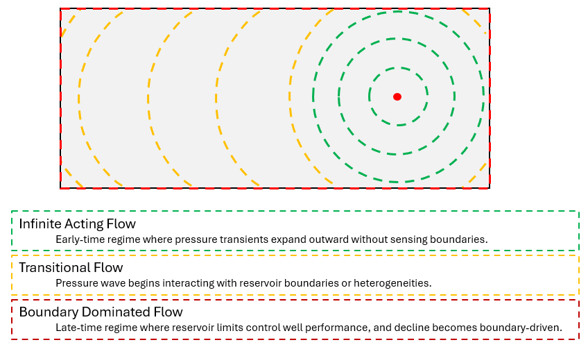
Figure 1: Flow regimes around a vertical well. Schematic illustration of pressure propagation from a vertical well, showing the progression from infinite-acting radial flow (green), through transitional flow (yellow), to boundary-dominated flow (red), as the pressure disturbance encounters the effective drainage boundaries and their influence becomes established.

Transitional behavior develops as reservoir boundaries, neighboring wells, or changes in reservoir properties begin to influence the pressure response. During this period, the observed behavior may depart from the preceding transient-flow trend without yet exhibiting a fully developed boundary-dominated response. Boundary-dominated flow is established when the effective drainage limits govern the overall depletion behavior represented by the model.

Reservoir depletion occurs during both transient and boundary-dominated flow. The distinction is that, during transient flow, the region affected by production continues to expand, whereas boundary-dominated behavior reflects withdrawal from an established drainage volume. In a closed volumetric system, this late-time response provides a stronger basis for estimating connected hydrocarbons in place. The time required to reach boundary-dominated flow depends on reservoir diffusivity, well configuration, and drainage dimensions; the flow regime therefore cannot be established from elapsed production time alone.

Effective drainage boundaries may be associated with geological barriers or with interactions between producing wells. A sealing fault can form a physical no-flow boundary by preventing flow across the fault plane. In contrast, a flow divide may develop between neighboring producing wells without a physical barrier in the reservoir. Such a divide separates the regions supplying the wells and may shift as their relative production rates and flowing pressures change. An interference-related boundary should therefore be treated as a fixed no-flow boundary only where that approximation is consistent with the model assumptions and operating conditions.

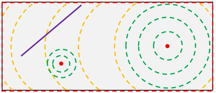
Figure 2: Effects of faults and well interference on drainage boundaries. Sealing faults can establish physical no-flow boundaries, while neighboring producing wells can create flow divides that separate their drainage regions without a geological barrier. These interference-related boundaries may shift as operating conditions change, affecting pressure propagation, flow regimes, and well performance.

Flow-regime identification is particularly important in low-permeability reservoirs, where hydraulically fractured wells may remain in transient flow for a substantial part of their production history. A smooth decline extending over several years may still reflect continued pressure propagation rather than boundary-dominated depletion of an established drainage volume. Diagnostic behavior should therefore be examined before conclusions are drawn about reservoir size or long-term recovery. A long production record, by itself, does not demonstrate that boundary-dominated flow has been reached.

Reliable bottomhole flowing-pressure data are also essential for distinguishing reservoir depletion from changes in operating conditions. Bottomhole flowing pressure may be measured directly or calculated from surface measurements using wellbore geometry, produced-fluid properties, temperature, and flow conditions. When calculated pressures are used, frictional pressure losses and the hydrostatic pressure contribution of fluids in the wellbore must be represented adequately.

For example, liquid buildup can increase bottomhole flowing pressure even when wellhead pressure remains constant. The resulting reduction in pressure drawdown can lower the production rate without a corresponding change in reservoir flow capacity. If this effect is not captured in the pressure calculation, the production decline may be incorrectly attributed to reservoir depletion. Particular attention is therefore required when liquid holdup changes or unstable multiphase flow makes the calculated bottomhole pressure uncertain.

Rate and pressure data must also represent compatible time intervals and operating conditions. A production rate measured during a flowing period should not be paired with a pressure recorded during shut-in or under a different operating condition. Similarly, averaged rate and pressure values should be reviewed carefully when significant operating changes occur within the averaging period. Inconsistent rate-pressure pairing can distort the normalized response and lead to an incorrect interpretation of reservoir behavior.

The parameters obtained from an analysis depend on the information contained in the observed response. A combination of permeability and fracture dimensions may be constrained more strongly by transient data than either parameter individually. Boundary-dominated data may provide a better estimate of the effective connected volume while leaving the detailed drainage geometry uncertain. The reliability of each estimated parameter should therefore be assessed in relation to the observed flow regimes and the assumptions required by the selected model.

The interpretation should also be evaluated against independent information, including geology, completion design, fluid properties, and available pressure measurements. A satisfactory match indicates that the selected model is consistent with the observed production response, but it does not establish that the reservoir description is unique. Confidence is strengthened when the interpretation is supported by both the production diagnostics and the broader understanding of the well and reservoir.

1.2. Conventional Decline Analysis and Fetkovich Typecurves

Conventional Arps decline analysis provides a practical description of production behavior using an initial rate, an initial decline rate, and a decline exponent. Exponential decline has a constant fractional decline rate. Hyperbolic decline has a fractional decline rate that decreases with time, with harmonic decline forming a particular member of that family. These relationships provide a concise basis for forecasting rates and cumulative recovery to a defined time or abandonment condition.

The method is attractive because it requires relatively little reservoir information. A representative production segment can be fitted without specifying permeability, net pay, porosity, or drainage geometry. We use this simplicity to establish a production trend and an initial forecasting reference. The forecast remains conditional on the selected interval and on the assumption that its behavior is representative of future production. An empirical decline exponent describes curve shape; it is not a unique indicator of reservoir drive mechanism, fracture geometry, or hydrocarbons in place.

Conventional decline extrapolation is most defensible when the well is in boundary-dominated flow and its operating conditions are reasonably stable. Rate-only analysis cannot explicitly separate the influence of a changing flowing pressure from depletion. It can therefore overestimate or underestimate future recovery when compression, choke changes, lift modifications, or production restrictions alter the observed trend. Transient-dominated production presents an additional limitation because the decline may not yet reflect depletion of a finite, established drainage volume.

Fetkovich typecurve analysis introduced a connection between transient-flow theory and empirical decline forecasting. The transient portion is derived from analytical reservoir-flow solutions, while the depletion portion incorporates the Arps decline family. The reference curves express rate and time in dimensionless form so that field production data can be compared with a common set of model responses. This makes the transition from transient behavior to depletion visible within a single interpretation framework.

The original transient model represents a well producing at constant sandface pressure in a homogeneous, bounded reservoir containing a slightly compressible single-phase fluid. Its late-time analytical response is exponential, which provides the connection to the empirical decline family. Later normalized-data formulations extend the treatment of flowing-pressure variation, but these should be distinguished from the assumptions of the original constant-pressure typecurves.

We use Fetkovich analysis to examine whether the available history contains transient behavior, an identifiable transition, and a depletion trend suitable for forecasting. A transient-only match cannot independently establish reservoir size, even when the displayed typecurve family is indexed by a dimensionless drainage parameter. Multiple matches may represent the same early-time behavior. Reservoir-volume conclusions require additional constraints or a sufficiently developed boundary response. Fetkovich analysis therefore provides an important link between conventional decline forecasting and analytical production interpretation. It adds flow-regime context to the decline history while retaining a familiar empirical representation of late-time production. Where operating pressure varies substantially or gas properties change significantly during depletion, pressure-normalized analytical methods provide a more suitable framework for incorporating those effects explicitly.

1.3. Blasingame Typecurve Analysis

Blasingame analysis was developed to interpret production histories in which both rate and flowing pressure vary. Its foundation is the use of analytical reservoir responses together with pressure-normalized production and an appropriate production-history time function. This allows the observed performance to be related more directly to reservoir behavior than is possible with a rate-time trend alone. The approach also incorporates transformations needed to account for pressure-dependent gas properties.

Pressure normalization relates the production rate to the drawdown applied at the well. For a slightly compressible liquid, the rate is divided by the difference between initial reservoir pressure and bottomhole flowing pressure. Gas analysis uses the corresponding pseudopressure difference. The purpose is to account for the changing pressure condition under which production occurs. This normalized rate should not be confused with a productivity index referenced to average reservoir pressure; the two quantities use different pressure references and serve different purposes.

Material-balance time relates cumulative withdrawal to the current production rate. It provides a coordinate for interpreting variable-rate depletion behavior rather than treating all production histories as equivalent when plotted against elapsed time. For gas, material-balance pseudotime additionally accounts for changing fluid properties as reservoir pressure declines. These transformations must remain consistent with the assumptions of the analysis. Pressure normalization alone does not remove the influence of all preceding rate changes or make an arbitrary operating history equivalent to a constant-pressure test.

The Blasingame presentation typically includes normalized rate, rate integral, and rate integral derivative. The companion functions improve the visibility of diagnostic behavior and help assess whether one model describes the complete response. Under the applicable depletion assumptions, the transient branches converge toward a single analytical harmonic stem in the transformed coordinates. This harmonic appearance results from the transformation; it does not mean that the well necessarily follows an Arps harmonic decline with elapsed time.

Gas-property treatment is a major part of the method's physical basis. As pressure decreases, gas viscosity, deviation factor, and compressibility change, affecting both flow and storage. Pseudopressure accounts for pressure-dependent mobility in the flow formulation, while pseudotime addresses the changing storage and diffusivity terms. Where the transformation uses properties at average reservoir pressure, the interpretation is coupled to the assumed gas in place and may require iteration. The calculation details are introduced in the method-specific sections.

We interpret the transient response using a model appropriate to the well and completion. Depending on that model and the available flow regimes, the analysis may constrain formation flow capacity, skin, or fracture-related properties. A supported depletion response can provide information on connected hydrocarbons in place and drainage volume. These quantities are not necessarily all identifiable from one production history, and their reliability depends on the input properties and the quality of the match.

The rate integral smooths short-term scatter, but it does not create independent measurements. Its derivative is also derived from the same production and pressure records. We therefore use agreement among the plotted functions as a consistency check and examine the original history when discontinuities or systematic mismatches occur. A visually smooth integral response cannot compensate for incorrect pressures, missing cumulative production, or a model that does not represent the producing system.

1.4. Agarwal–Gardner and Complementary Methods

Agarwal–Gardner analysis also combines production decline interpretation with analytical well-test concepts. It builds on the earlier typecurve developments and provides another representation of normalized production behavior. Its purpose is to identify the transition from transient flow to depletion and relate that response to well and reservoir properties. Like Blasingame analysis, it relies on appropriate pressure and time transformations to interpret variable operating conditions and the changing properties of gas.

A distinguishing feature is its use of dimensionless variables based on conventional well-test definitions rather than the decline scaling used in the Fetkovich-style presentation. The method includes rate-time, rate-cumulative, and cumulative-time representations, together with derivative diagnostics. These alternatives allow the same history to be examined from different perspectives. The details of derivative and integral-derivative displays can differ between implementations and should be defined in the corresponding calculation section.

We use the rate-time response to assess flow-regime development and the consistency of the selected model. The rate-cumulative representation provides a complementary depletion perspective and can support hydrocarbons-in-place estimation when the required conditions are satisfied. Its transformed variables must be distinguished from a simple plot of raw rate against cumulative production. Extrapolating an uncorrected production trend does not provide the same physical interpretation as an analytical depletion relationship that accounts for flowing pressure and fluid properties.

Blasingame and Agarwal–Gardner analyses should be viewed as complementary analytical methods. Differences in scaling and diagnostic presentation can make particular features easier to recognize in one plot than another. However, they use the same underlying production history and related reservoir-flow principles. Agreement between them supports consistency, while disagreement prompts a review of the data, transformations, selected flow regime, and model assumptions. It should not automatically be resolved by selecting whichever method yields the preferred volume.

Normalized pressure integral analysis provides a related pressure-based representation of the production response. Integrating a normalized response reduces the influence of short-term scatter and supports comparison with analytical typecurves. The method belongs to the same broader development in which well-test processing concepts were adapted to routine production records. As with rate integrals, the resulting smoothness improves interpretation but does not remove systematic data errors or establish a unique reservoir model.

Flowing material balance addresses connected reservoir inventory from a depletion perspective. Conventional material balance relates cumulative production to changes in average reservoir pressure and fluid properties. Flowing material balance uses production rates and flowing pressures together with an appropriate reservoir-to-well flow relationship to obtain a depletion interpretation. It accounts for the distinction between average reservoir pressure and flowing bottomhole pressure; the two pressures are not interchangeable.

We apply flowing material-balance concepts where the production history supports the required depletion assumptions. For a volumetric system, the objective is to estimate the reservoir volume contributing to production and then evaluate recovery under defined future conditions. Aquifer influx, changing connectivity, or strong mobility changes can invalidate a simple closed-system interpretation. The inferred volume must be consistent with the physical model and the portion of the reservoir sampled by the available history.

1.5. Using the Methods Together

The interpretation is guided by the engineering question being addressed. If the objective is to forecast production under an established operating strategy, conventional decline analysis may be used as a reference. If flow regimes or reservoir and completion properties are to be evaluated, an analytical interpretation appropriate to the well and reservoir should be selected. If connected hydrocarbons in place are to be estimated, sufficient depletion information or independent constraints must be available to support the estimate. The analysis method should therefore be selected according to the objective and the available evidence.

The relevant physical processes must also be represented adequately by the analytical model. In many basic formulations, single-phase flow, constant rock and completion properties, and volumetric depletion are assumed. Where water influx, well interference, pressure-dependent permeability, changing fracture conductivity, or multiphase mobility effects are significant, an extended formulation or numerical model may be required. A gas reservoir with significant condensate banking, for example, cannot automatically be treated as a constant-mobility, single-phase system simply because gas dominates the produced volume.

Parameter estimation should be distinguished from forecasting. Through history matching, the observed response is reproduced under a selected set of model assumptions. For forecasting, future operating pressures or rate constraints, completion conditions, and an abandonment criterion must also be specified. Different recovery estimates may be obtained when these assumptions are changed, even if the initial connected hydrocarbons in place remain unchanged. By treating parameter estimation and forecasting as separate stages, the basis of each forecast can be assessed more clearly and alternative operating strategies can be compared consistently.

A common framework for the following sections is established by the methods introduced here. First, the flow behavior represented by the data is identified. The parameters supported by that behavior are then estimated, and forecasts are developed under explicitly defined operating assumptions. Each plotting function, its required inputs, and the calculation sequence will be explained through detailed equations and worked examples. The physical meaning and applicability of these calculations are introduced here to provide a foundation for their subsequent use.

2. Decline Curve Analysis (DCA)

2.1. Introduction

As introduced in Section 1, production analysis may be used for both forecasting and reservoir characterization. Conventional DCA primarily addresses the forecasting objective. An observed production trend is represented by a mathematical relationship and extrapolated under specified assumptions about future operating conditions.

DCA is widely used to forecast well production, estimate remaining recoverable volumes, and support reserves evaluation. Among the available formulations, the classical Arps equations remain a foundation of conventional decline analysis. Production decline is described using three parameters: the production rate at the beginning of the selected decline period, the initial nominal decline rate, and the decline exponent.

The principal advantage of the Arps method is its simplicity. A production trend can be characterized without explicitly specifying reservoir permeability, drainage geometry, skin, or hydraulic-fracture properties. This makes the method useful when production history is available but detailed reservoir information is limited.

Its applicability nevertheless depends on the behavior represented by the selected production interval. The strongest basis for conventional Arps forecasting is established boundary-dominated flow under reasonably stable operating conditions. Application to transient-dominated production may provide a satisfactory mathematical fit, but extrapolation beyond the observed period requires additional justification.

2.2. General Arps Formulation

The nominal decline rate is defined as the instantaneous fractional rate of decrease in production:

$$\begin{equation} \label{eq:nominal-decline} D(t) = -\frac{1}{q(t)}\frac{dq(t)}{dt} \end{equation}$$

In the Arps formulation, the nominal decline rate varies with time according to:

$$\begin{equation} \label{eq:arps-decline-rate} D(t) = \frac{D_i}{1 + bD_it} \end{equation}$$

Integration gives the general hyperbolic rate equation:

$$\begin{equation} \label{eq:arps-general} q(t) = \frac{q_i}{\left(1 + bD_it\right)^{1/b}} \end{equation}$$

where:

• $q(t)$ is production rate at elapsed time $t$
• $q_i$ is production rate at the beginning of the selected decline period
• $D_i$ is initial nominal decline rate
• $b$ is Arps decline exponent
• $t$ is elapsed time from the beginning of the decline period

The time origin is the beginning of the analyzed decline segment and does not necessarily coincide with the well's first production date. Similarly, $q_i$ is the rate associated with that segment and should not automatically be interpreted as the well's initial production rate.

The units of $D_i$ must be consistent with the time units used in the equation. For example, if time is expressed in years, the nominal decline rate must be expressed in reciprocal years. The product $D_it$ is dimensionless.

The exponential case is obtained as the limit of Eq. \eqref{eq:arps-general} as $b$ approaches zero. It should not be evaluated by directly substituting $b = 0$ into that equation.

2.3. Classical Arps Decline Models

The classical Arps family consists of exponential, hyperbolic, and harmonic decline. Their main distinction is how the nominal decline rate changes with time.

2.3.1. Exponential Decline

For exponential decline, $b = 0$, and the production-rate relationship becomes:

$$\begin{equation} \label{eq:arps-exponential} q = q_i e^{-D_it} \end{equation}$$

The nominal decline rate remains constant:

$$\begin{equation} \label{eq:exponential-decline-rate} D(t) = D_i \end{equation}$$

Consequently, the same fractional reduction in production occurs over equal time intervals. Although the Arps framework was developed empirically, exponential decline also has a theoretical basis for a bounded reservoir containing a slightly compressible single-phase fluid produced at constant bottomhole flowing pressure under the appropriate assumptions. Conventional DCA, however, does not require that physical model to be specified when the curve is fitted.

2.3.2. Hyperbolic Decline

For classical hyperbolic decline, $0 < b < 1$ and:

$$\begin{equation} \label{eq:arps-hyperbolic} q = \frac{q_i}{\left(1 + bD_it\right)^{1/b}} \end{equation}$$

The nominal decline rate decreases with time according to Eq. \eqref{eq:arps-decline-rate}. Production therefore declines rapidly at first and more gradually at later time.

2.3.3. Harmonic Decline

Harmonic decline is the limiting classical hyperbolic case for which $b = 1$:

$$\begin{equation} \label{eq:arps-harmonic} q(t) = \frac{q_i}{1 + D_it} \end{equation}$$

The corresponding nominal decline rate is:

$$\begin{equation} \label{eq:harmonic-decline-rate} D(t) = \frac{D_i}{1 + D_it} \end{equation}$$

2.4. Applicability and Limitations of Classical Arps DCA

Classical Arps analysis is most applicable to production during boundary-dominated flow under reasonably stable operating conditions. It is not a general transient-flow reservoir model, and a declining production trend alone does not demonstrate that its underlying assumptions have been satisfied.

Changes in bottomhole flowing pressure, choke settings, compression, artificial lift, facility constraints, or liquid loading may alter production independently of reservoir depletion. Workovers, refracturing, and offset-well interference may also change well performance or the reservoir pressure response. Production history should therefore be reviewed before decline-curve fitting, and periods with substantially different operating conditions may need to be analyzed separately.

2.4.1. What an Arps Match Determines

An Arps match provides an empirical description of production-rate behavior through three decline parameters: $q_i$, $D_i$, and $b$. Once these parameters have been established, the fitted relationship can be extrapolated to estimate:

• Future production rates and cumulative production.
• Time to a specified economic or operational limit.
• Remaining recoverable volume and estimated ultimate recovery (EUR).

These estimates are conditional on the selected decline model and future operating assumptions. They may support reserves evaluation, but recoverable volumes are not automatically classified as reserves without consideration of the applicable commercial and project criteria.

The fitted parameters are decline-model parameters rather than independently determined reservoir properties. Although Arps relationships can have a physical basis under specific assumptions, a conventional rate-time match does not uniquely determine permeability, skin, drainage area, hydrocarbons in place, or fracture properties such as half-length and dimensionless conductivity. These properties influence production, but their individual contributions generally cannot be separated through an Arps match alone.

Arps DCA is therefore primarily used to forecast production based on the continuation of an established trend. Identification of the controlling flow regime and interpretation of reservoir and completion properties require complementary methods, such as pressure-transient analysis, rate-transient analysis, material balance, or analytical and numerical reservoir modeling. A satisfactory decline match does not, by itself, establish a unique physical explanation of well performance.

2.4.2. Forecast Uncertainty

Different combinations of $q_i$, $D_i$, and $b$ may provide similarly acceptable matches over a limited historical interval while producing substantially different long-term forecasts. EUR is particularly sensitive to the extrapolated production tail, which depends on the decline exponent, terminal decline rate, abandonment criterion, and forecast duration.

For the same $q_i$ and $D_i$, a larger $b$-value produces a slower late-time decline and greater forecast cumulative production. Consequently, relatively small differences in the selected exponent can materially affect EUR, especially when much of the estimated recovery lies beyond the observed production history.

An acceptable statistical fit should therefore be supported by an engineering assessment of the operating history, expected flow regime, and plausible long-term performance. Where several parameter combinations are reasonable, forecast sensitivity should be evaluated rather than relying on a single fitted curve.

2.4.3. Application During Transient Flow

During transient flow, the pressure disturbance continues to propagate through the reservoir, progressively extending the region affected by production. Depletion is occurring, but the production response is not yet controlled by an established drainage volume. These conditions are particularly important in low-permeability reservoirs, where hydraulically fractured horizontal wells may remain in transient flow for months or years.

An Arps equation may provide a satisfactory match to this history, but the fitted parameters describe the observed transient trend rather than demonstrated boundary-dominated behavior. Extrapolation far beyond the available data may therefore produce a forecast with limited physical support.

The prevailing flow regime should be assessed before classical Arps parameters are relied upon for long-term forecasting. Where boundary-dominated flow has not been established, the forecast should be treated as an empirical projection and evaluated using additional constraints, such as analytical or numerical models, diagnostic analysis, and relevant analog performance.

Arps DCA primarily addresses the forecasting question:

• If the historical production decline continues according to the selected mathematical decline model, what future production profile and cumulative recovery should be expected?

It does not independently answer the reservoir-characterization questions:

• Why is the well declining in this manner?
• What flow regime is controlling the observed production response?
• What reservoir, well, and completion properties are responsible for the observed behavior?

Answering these questions requires reservoir-engineering methods that incorporate a physical representation of fluid flow, such as Pressure Transient Analysis (PTA), Rate Transient Analysis (RTA), analytical reservoir models, numerical reservoir simulation, material-balance methods, and physics-based typecurve analysis. These techniques relate measured pressure and production responses to reservoir and completion properties through the governing equations of fluid flow.

Accordingly, classical Arps DCA should primarily be viewed as a production-forecasting and reserves-estimation methodology, rather than as a stand-alone reservoir-characterization technique.

Its strength lies in its ability to describe and extrapolate an established production trend with relatively few parameters. Its limitation is that a satisfactory mathematical match to production history does not necessarily constitute a unique physical interpretation of reservoir behavior.

2.5. Transition from Arps DCA to Typecurve Analysis

The limitations of classical Arps DCA during transient flow provide a natural transition to production typecurve analysis. Although an empirical decline equation may reproduce an observed production trend, the controlling flow regime cannot be identified from the quality of that fit alone.

A major advancement was introduced through Fetkovich typecurve analysis, in which analytical solutions for transient reservoir flow were combined with the classical Arps decline relationships for boundary-dominated production. Transient behavior, the transition toward depletion, and established boundary-dominated decline could therefore be examined within a common framework.

With this development, production analysis was extended beyond empirical curve fitting. The shape of the measured response and its alignment with theoretical typecurves could be used to assess the underlying flow behavior and determine whether boundary-dominated flow had been established. This distinction is important because the reservoir properties and connected volumes that can be estimated depend on the flow regimes represented in the available history.

The framework was subsequently extended through the Blasingame and Agarwal–Gardner methodologies. In these methods, pressure-normalized rate functions are combined with material-balance time or material-balance pseudotime to account for changing production conditions. For gas reservoirs, pseudopressure and pseudotime are used to incorporate pressure-dependent fluid properties more rigorously. Production histories with variable rates and flowing pressures can consequently be interpreted within the assumptions of the selected analytical model.

The progression is therefore from empirical forecasting toward increasingly detailed physical interpretation. Classical Arps DCA is used to describe and extrapolate an established decline trend. Through Fetkovich analysis, that trend is placed within the context of transient and boundary-dominated flow. In modern typecurve and rate-transient analysis, pressure and production history are interpreted together using models that represent reservoir geometry, well configuration, and fluid-flow behavior.

Arps DCA remains a useful forecasting method within its applicable range. When the objective extends to identifying flow regimes or estimating reservoir and completion properties, it should be complemented by methods that explicitly relate the production response to the governing reservoir physics.

The progression can therefore be viewed conceptually as:

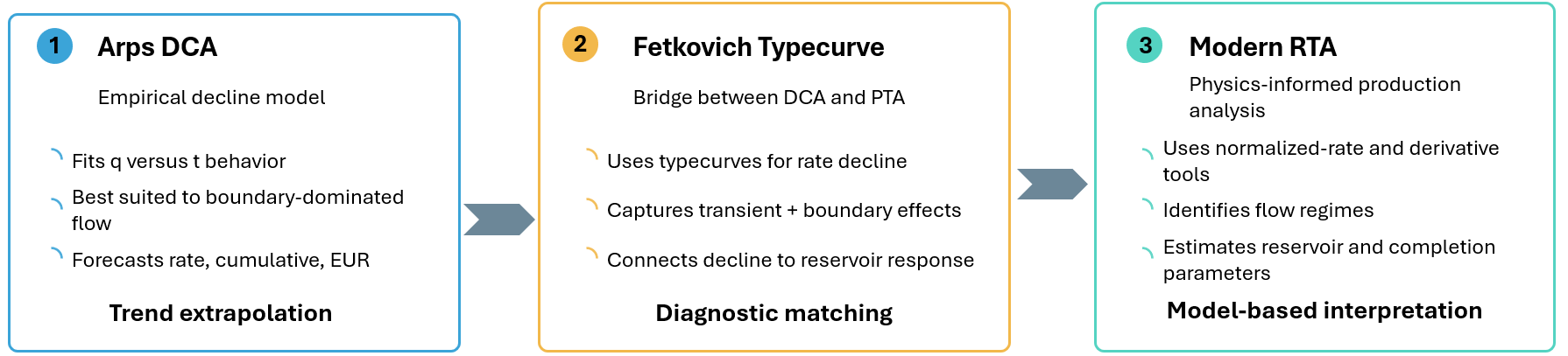
Figure 3: Conceptual progression from Arps DCA (trend extrapolation), through Fetkovich typecurves (diagnostic matching), to modern RTA (model-based interpretation).

3. Dry Gas Reservoirs Material Balance

Gas typecurve analysis commonly uses pseudotime to account for the pressure-dependent variation of gas viscosity and total system compressibility during reservoir depletion. Pseudotime calculation therefore requires a representative pressure history at which these properties can be evaluated. For conventional gas reservoirs, this representative pressure is commonly taken as the average reservoir pressure. Because average reservoir pressure is rarely measured continuously, it is often estimated from cumulative production using material balance. Material balance is therefore included as a complementary component of the typecurve analysis workflow, providing the average-pressure history required for pseudotime evaluation.

Material balance is one of the fundamental principles used to describe and evaluate reservoir performance. It is a macroscopic application of the conservation-of-mass principle in which the reservoir, or the portion of the reservoir in pressure communication with the producing wells, is treated as a single control volume. Rather than describing the detailed movement of fluids at individual locations, material balance accounts for the overall quantities of oil, gas, and water initially present, together with fluids produced from or introduced into the reservoir through injection or natural water influx. Accordingly, the total mass remaining in the reservoir at any given time is equal to the mass originally present, plus the mass introduced into the system, minus the mass withdrawn through production. This relationship may be expressed mathematically as:

$$\begin{equation} \label{eq:mass-balance} M_{remaining} = M_{initial} + M_{injected} - M_{produced} \end{equation}$$

A useful physical interpretation of material balance is that the net volume of fluids withdrawn from the reservoir must be balanced by corresponding changes within the reservoir system. As reservoir pressure declines, oil, gas, and connate water may expand, while rock compaction may reduce the available pore volume. Natural water influx and fluid injection may also replace part of the withdrawn volume and provide pressure support. Material balance combines these contributions within a consistent reservoir-volume framework by relating fluid withdrawal to fluid expansion, pore-volume change, and external fluid support. This interpretation is particularly useful because production and injection data are commonly measured and reported as fluid volumes.

For the dry-gas reservoir considered in this manual, these physical changes are illustrated schematically in Figure 4. At the initial condition, the reservoir pore volume is occupied by the original gas and connate water. As the reservoir is depleted from the initial pressure, $p_i$, to a lower average pressure, $p$, gas and water may be produced, the remaining fluids expand, and the reservoir pore volume may contract. Natural water influx and water injection may replace part of the withdrawn fluid volume and provide additional pressure support. The material-balance relationship accounts for these effects by connecting the initial fluid inventory with the fluids remaining in the reservoir, the cumulative volumes produced or injected, and the change in pore volume during depletion.

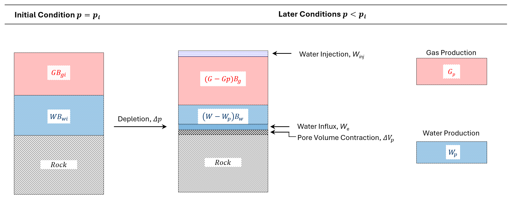
Figure 4: Schematic reservoir volume representation of dry gas material balance between the initial and depleted conditions, including gas and water production, natural water influx, water injection, and pore volume contraction.

The physical contributions described above can be combined into a single material-balance relationship. For a dry-gas reservoir, the expansion of the original fluids, pore-volume contraction, and external water support must collectively account for the reservoir volume withdrawn through gas and water production.

The following derivation assumes an isothermal, pressure-connected reservoir in which the hydrocarbon fluid remains in the gas phase at reservoir conditions. Gas injection is neglected; if gas is injected, cumulative gas production should be replaced by cumulative net gas withdrawal. Natural water influx, $W_e$, is expressed in reservoir-volume units, while produced and injected water are converted to reservoir conditions using $B_w$. All quantities must be expressed in consistent units.

3.1. Governing Material-Balance Relationship

For a dry gas reservoir that may experience natural water influx, water injection, water production, and pore volume contraction, the material balance relationship may first be written in reservoir volume form. At the initial condition, the reservoir pore volume is occupied by the original gas and connate water. At a later pressure, the reservoir contains the remaining gas and connate water, together with any water added through injection or natural influx. The reduction in pore volume that occurs during reservoir depletion must also be included. Therefore,

$$\begin{equation} \label{eq:mb-reservoir-volume} GB_{gi} + WB_{wi} = \left(G - G_p\right)B_g + \left(W - W_p + W_{inj}\right)B_w + W_e + \Delta V_p \end{equation}$$

Here, $W_e$ is the cumulative natural water influx expressed in reservoir volume units, and $\Delta V_p$ is the reduction in reservoir pore volume between the initial and current conditions:

$$\begin{equation} \label{eq:pore-volume-reduction} \Delta V_p = V_{pi} - V_p \end{equation}$$

With this sign convention, $\Delta V_p$ is positive when the pore volume contracts during pressure depletion.

Expanding the terms on the right-hand side and collecting the initial- and current-condition quantities gives

$$\begin{equation} \label{eq:mb-rearranged} G\left(B_g - B_{gi}\right) + W\left(B_w - B_{wi}\right) + \Delta V_p + W_e = G_pB_g + \left(W_p - W_{inj}\right)B_w \end{equation}$$

The first two terms on the left-hand side represent the expansion of the original gas and connate water, respectively. The pore volume term represents the contribution associated with reservoir compaction, while $W_e$ represents pressure support provided by natural water influx. On the right-hand side, $G_pB_g$ is the reservoir volume of the produced gas, and $\left(W_p - W_{inj}\right)B_w$ is the net water withdrawal evaluated at reservoir conditions.

To express the material-balance relationship more compactly, define the gas, water, and pore-volume expansivities as

$$\begin{equation} \label{eq:Eg} E_g = B_g - B_{gi} \end{equation}$$

$$\begin{equation} \label{eq:Ew} E_w = B_w - B_{wi} \end{equation}$$

and

$$\begin{equation} \label{eq:Ef} E_f = \frac{\Delta V_p}{V_{pi}} \end{equation}$$

From the definition of pore volume expansivity,

$$\begin{equation} \Delta V_p = V_{pi}E_f \end{equation}$$

Substituting these definitions into the rearranged material-balance relationship gives the expansivity form

$$\begin{equation} \label{eq:mb-expansivity} GE_g + WE_w + V_{pi}E_f + W_e = G_pB_g + \left(W_p - W_{inj}\right)B_w \end{equation}$$

In the expansivity form, gas expansion, connate water expansion, pore volume contraction, and natural water influx collectively account for the reservoir volume removed through gas production and net water production.

To recast the material-balance equation in a pressure-based form analogous to the conventional $p/z$ relationship, the expansion terms must first be related to reservoir pressure decline. Beginning with the definition of water compressibility:

$$\begin{equation} \label{eq:cw} c_w = -\frac{1}{B_w}\frac{dB_w}{dp} \end{equation}$$

Integrating from $p_i$ to $p_{avg}$ relates the change in water formation volume factor to the pressure decline, where $\Delta p = p_i - p_{avg}$. For constant water compressibility, the resulting expression has an exponential form. Because $c_w\Delta p$ is generally small, the first-order approximation $e^x - 1 \approx x$ may be applied. The water expansivity is therefore approximated as

$$\begin{equation} \label{eq:Ew-approx} E_w = B_w - B_{wi} \approx B_{wi}c_w\Delta p \end{equation}$$

Accordingly, the connate water expansion term becomes

$$\begin{equation} WE_w = WB_{wi}c_w\Delta p \end{equation}$$

A similar development applies to the pore-volume contraction term. Assuming constant formation compressibility and a sufficiently small value of $c_f\Delta p$, the pore-volume expansivity may be approximated as

$$\begin{equation} \label{eq:Ef-approx} E_f = c_f\Delta p \end{equation}$$

To simplify the material balance equation further, the initial pore volume and connate water volume are expressed in terms of the original gas in place. At initial conditions,

$$\begin{equation} GB_{gi} = V_{pi}\left(1 - S_{wi}\right) \end{equation}$$

so that

$$\begin{equation} V_{pi} = \frac{GB_{gi}}{1 - S_{wi}} \end{equation}$$

The initial connate-water volume is

$$\begin{equation} WB_{wi} = V_{pi}S_{wi} \end{equation}$$

which gives

$$\begin{equation} W = \frac{S_{wi}}{1 - S_{wi}}\frac{GB_{gi}}{B_{wi}} \end{equation}$$

Using these expressions for the initial pore volume and connate-water volume in the general material-balance relationship introduced earlier, and collecting like terms, the equation can be rearranged into the following form:

$$\begin{equation} \label{eq:mb-normalized} \frac{B_g}{B_{gi}} - 1 + C_T\Delta p = \frac{G_pB_g}{GB_{gi}} + \frac{\left(W_p - W_{inj}\right)B_w - W_e}{GB_{gi}} \end{equation}$$

where $C_T$ is the effective rock and connate water compressibility correction, normalized to the initial gas-filled pore volume:

$$\begin{equation} \label{eq:CT} C_T = \frac{c_wS_{wi} + c_f}{1 - S_{wi}} \end{equation}$$

Note

The quantity $C_T$ should not be confused with the total system compressibility, $c_t$, used in the pseudotime calculation.

3.2. Corrected $p/z$ Relationship

The material balance relationship can now be written in a form analogous to the conventional $p/z$ equation. At constant reservoir temperature, the gas formation-volume-factor ratio is related to pressure and gas deviation factor by $B_g/B_{gi} = \left(z/p\right)/\left(z_i/p_i\right)$. Substituting this relationship into Eq. \eqref{eq:mb-normalized} and rearranging for $p/z$ gives

$$\begin{equation} \label{eq:pz-corrected} \frac{p}{z} = \frac{\frac{p_i}{z_i}\left(1 - \frac{G_p}{G}\right)}{1 - C_T\Delta p + \frac{\left(W_p - W_{inj}\right)B_w - W_e}{GB_{gi}}} \end{equation}$$

This expression represents a corrected $p/z$ material balance relationship that accounts for rock and connate-water expansion, water production, water injection, and natural water influx. When these additional effects are negligible, the denominator approaches unity and the equation reduces to the conventional volumetric dry gas $p/z$ relationship:

$$\begin{equation} \label{eq:pz-conventional} \frac{p}{z} = \frac{p_i}{z_i}\left(1 - \frac{G_p}{G}\right) \end{equation}$$

3.2.1. Physical Interpretation of the Correction Terms

The denominator of the corrected $p/z$ relationship is

$$\begin{equation} 1 - C_T\Delta p + \frac{\left(W_p - W_{inj}\right)B_w - W_e}{GB_{gi}} \end{equation}$$

Each term modifies the estimated $p/z$ according to whether it provides reservoir support or represents an additional fluid withdrawal. Pore volume contraction and connate water expansion are represented by the term $C_T\Delta p$. Because this term is subtracted from unity, these effects reduce the denominator and increase the corrected $p/z$. For a given cumulative gas production, this generally results in a higher estimated average reservoir pressure than that obtained from the conventional volumetric relationship.

Natural water influx and water injection have a similar directional effect. Both replace part of the volume withdrawn from the reservoir, reduce the denominator, and provide pressure support. Water production has the opposite effect: it represents an additional reservoir volume withdrawal, increases the denominator, and lowers the corrected $p/z$ and corresponding average reservoir pressure.

This interpretation may be summarized as follows: fluid expansion, pore-volume contraction, water influx, and water injection support reservoir pressure, whereas gas and water production contribute to reservoir depletion.

These additional pressure support and withdrawal terms make the corrected $p/z$ relationship more representative of actual reservoir behavior. However, they also make the equation implicit because the average reservoir pressure appears both directly and through pressure dependent quantities such as $z$, $B_w$, and $\Delta p$. Consequently, the corrected average pressure generally cannot be obtained by direct substitution and must be determined iteratively.

3.3. Numerical Solution of the Implicit Equation

A practical implementation first estimates the average reservoir pressure from the conventional volumetric $p/z$ relationship. The pressure-dependent correction terms are then evaluated at this trial pressure, and the corrected $p/z$ target is used to obtain an updated pressure from the PVT relationship. When the corrections are small, a single iteration may provide an adequate estimate, provided that the resulting material-balance residual is checked. Otherwise, the implicit equation should be solved using a bounded root-finding method, such as bisection or Brent's method, until both the pressure change and material-balance residual satisfy the specified tolerances. Newton–Raphson may converge more rapidly, but it requires a reliable initial estimate and derivative and is less robust when the relationship is strongly nonlinear or the PVT data are irregular.