Bottomhole Pressure Calculations
Estimating bottomhole pressure from measured wellhead pressure and temperature is an important task in petroleum engineering. Bottomhole pressures are required in most classical well-performance forecasting techniques such as rate-transient analysis (RTA), history matching using reservoir simulation, inflow-performance-relationship (IPR) estimation, and more.
Based on production data measured at the surface (i.e. surface rates, wellhead pressure, and wellhead temperature), and key properties describing the wellbore (i.e. a deviation survey describing the curvilinear shape of the well, wellbore diameter, and pipe roughness), we can estimate the bottomhole pressure by numerical integration of the pressure- and temperature gradient expression.
Multiphase flow in inclined pipe involves calculations of oil, gas, and water, which require an accurate fluid description (PVT). We achieve this by leveraging all the relevant capabilities of whitson+ seamlessly to provide accurate and consistent phase behavior in all calculations made on a particular well.
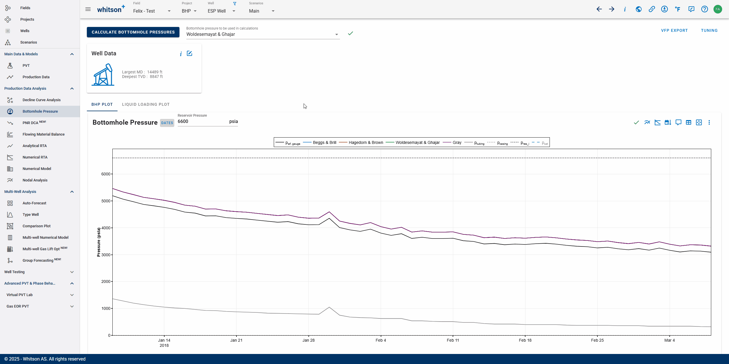
Currently Supported Correlations:
- Hagedorn and Brown (Liquid-Rich Wells)
- Beggs and Brill (Liquid-Rich Wells)
- Gray (Low-LGR Gas Wells)
- Woldesemayat and Ghajar (Liquid-Rich Wells)
1. Input
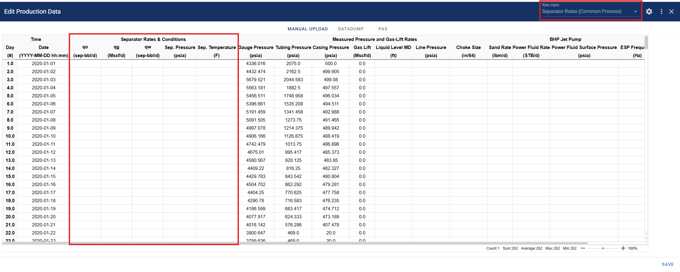
1.1. Production data
Daily production rates can be provided at stock-tank conditions or at separator conditions. If separator rates are provided, then the Common Process Conversion workflow can be used to generate stock-tank rates for the BHP calculations. In addition to production rates, one must also provide casinghead pressure and tubinghead pressure if tubing is installed. If the well is subjected to gas-lift, rod-pump assisted lift or ESP, lift-gas rates, liquid level in the annulus, and ESP frequency must be provided, respectively.
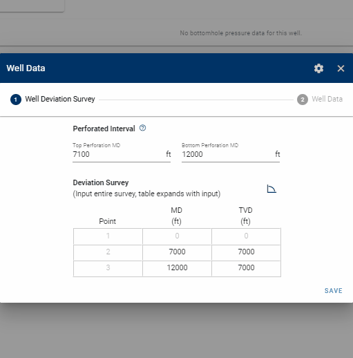
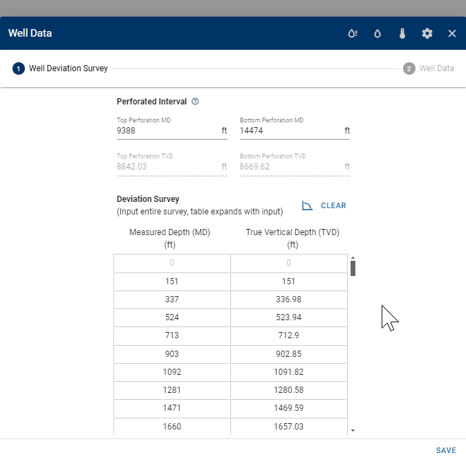
1.2. Well deviation survey
The well deviation survey describes the trajectory of the wellbore, and consists of a measured depth (MD) and calculated true vertical depth (TVD). The user can provide the full deviation survey of the well as the BHP module will sample the deviation survey backend to create the wellbore grid for BHP calculations. The perforated interval must be specified by providing the MD of the top and bottom perforations. The top perforation is also the reference depth at which the BHP is calculated.
Depth reference for all wellbore inputs
All depths in the BHP module are referenced to the deviation survey datum. In most cases, deviation surveys are referenced to KB, so tubing, casing, perforation, gauge, and valve depths should be entered as MD relative to KB. If your deviation survey uses a different datum, ensure all entered depths use that same datum (or convert them before input).
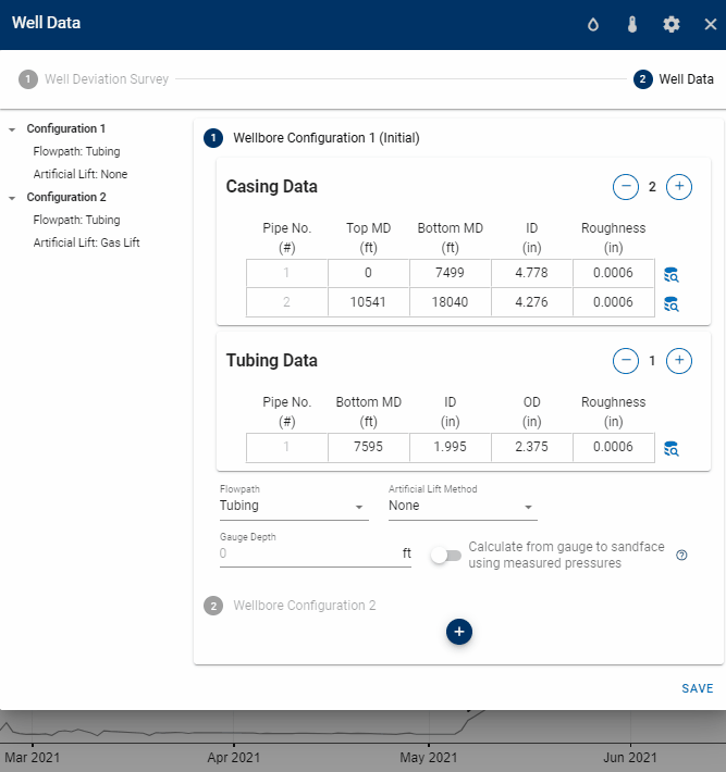
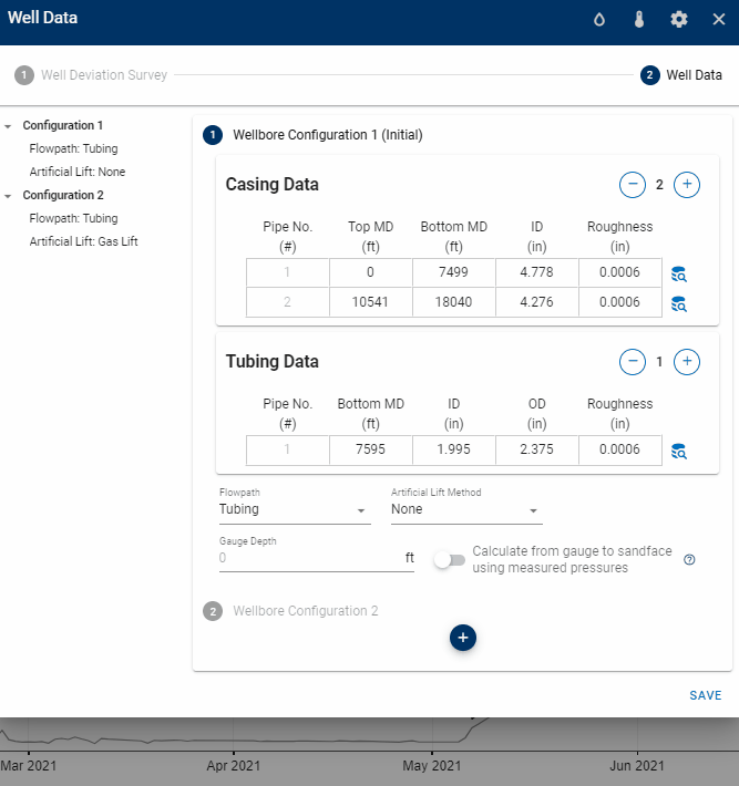
1.3. Well data
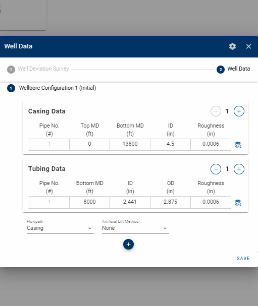
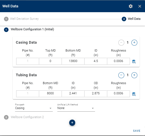
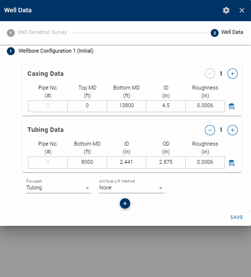
1.3.1. Casing and Tubing Data
The well data consists of properties for the tubing and casing string(s) relevant for pipe flow calculations (i.e., the depths of the different pipes, their diameters, and roughnesses). Multiple tubing and casing strings can be specified, where an API tubing and casing table is available to simplify the input of the pipe data.
Casing and tubing depth datum
Casing and tubing depths are interpreted as measured depth (MD) along the input deviation survey and use the same reference datum as the survey (typically KB). Enter all completion depths consistently with the deviation survey datum.
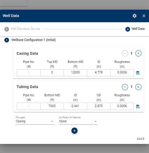
1.3.1.1. Concentric Tubing
For wells with concentric tubing, the input should represent the pipe geometry used for the active flow path.
If the well is flowing through the innermost tubing, enter the outer tubing as a casing string and enter the inner tubing as the actual tubing string. This allows the BHP calculation to use the correct flow path while still accounting for the surrounding pipe geometry.
When entering concentric tubing data:
- Add the larger, outer tubing under Casing Data.
- Add the smaller, inner tubing under Tubing Data.
- Use measured depth (MD) for all top and bottom depths.
- Use the appropriate ID, OD, and roughness values for each string.
- Set the Flowpath according to the string the well is actually flowing through.
Concentric tubing flow path
For most concentric tubing cases, the active flow path is through the inner tubing. In this case, the inner string should be entered as tubing, while the outer string should be entered as casing.
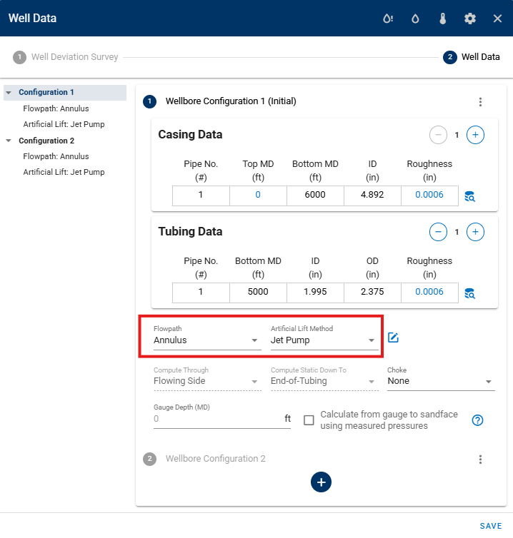
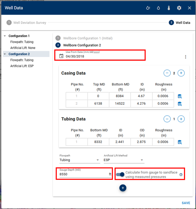
1.3.2. Multiple Wellbore Configurations
Multiple completion data sets, or wellbore configurations, can be specified. A date must be set to tell the BHP module from which date in the production time series each completion is used.
You can easily set the date for the new wellbore configuration graphically by clicking on the symbol adjacent to the date input field, as demonstrated in the .gif below. Then, simply align the vertical dashed line to the desired point in time when your new wellbore configuration should take effect.
Initial Wellbore Configuration Date
The first wellbore configuration is automatically set to begin from the first day of production.
1.3.3. Flow Paths
The user must also specify the flow path of the well stream for each wellbore configuration. The flow path can be:
- Tubing—well stream flows through a tubing string.
- Casing—well stream flows through the production casing.
- Annulus—well stream flows in the annular space between the tubing and production casing.
- Tubing & Annulus—well stream flows both through the tubing string and the annular space between the tubing and production casing. See the section on dual conduit flow for further details.
- Measured BHP—If pressures from a downhole gauge have been provided under the Gauge Pressure column in production data, one can instruct the BHP model to echo the measured BHP (applies to wells for which an accurate estimate of the BHP is available, and where the user wants to include that pressure in the resulting BHP profile for completeness).
- Unknown—Automatic selection of flow path depending on the casinghead pressure, tubinghead pressure, and associated well configuration. The following table summarizes the logic applied for the unknown flow path.
| Condition | Selected Flow Path |
|---|---|
| ≤ < and Tubing is Installed | Casing |
| ≤ < and Tubing is Installed | Tubing |
| < ≤ and Tubing is Installed | Tubing |
| < < and Tubing is Installed | Casing |
| Tubing is not Installed | Casing |
where is the pressure at standard conditions (14.696 psia).
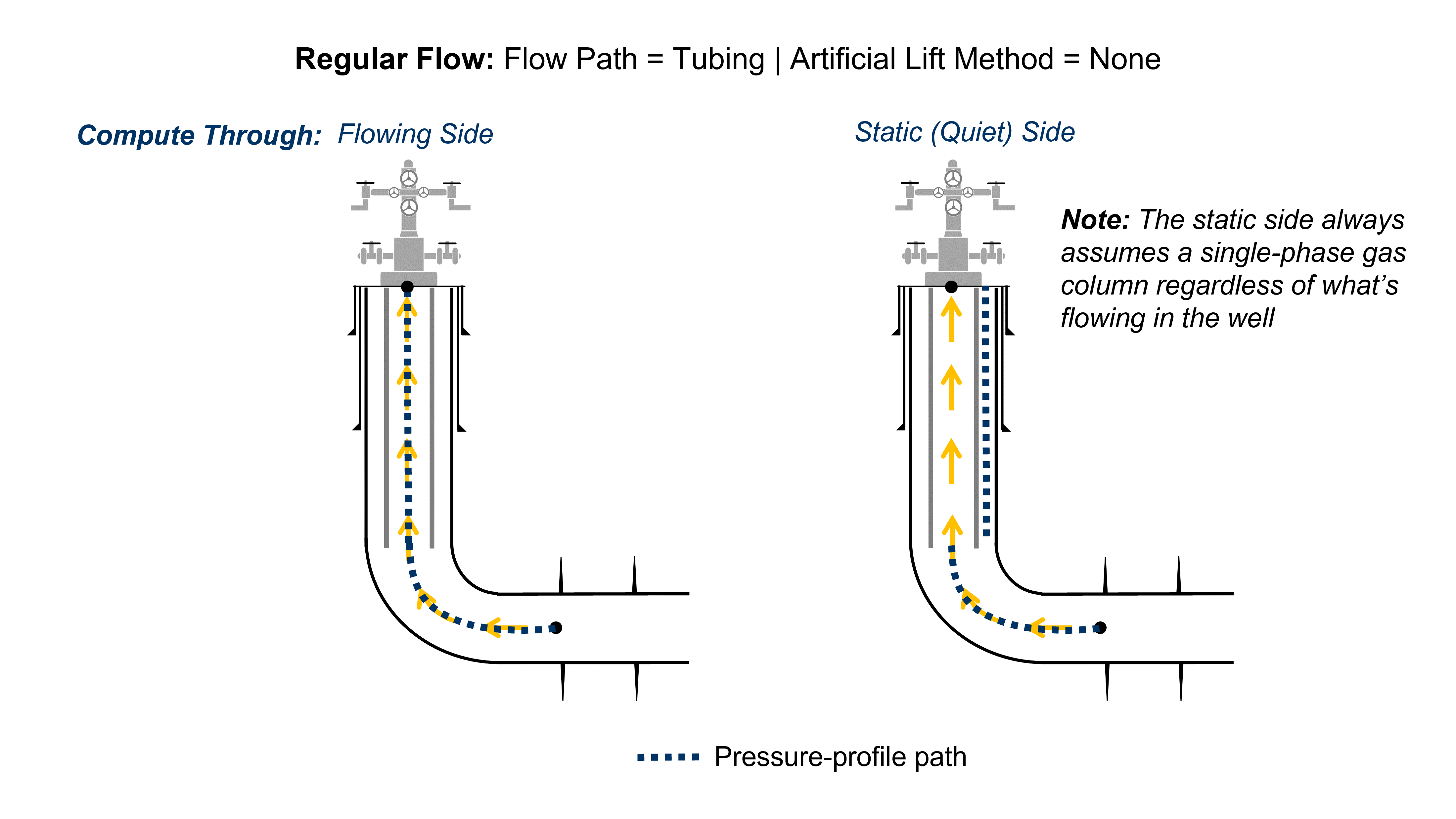
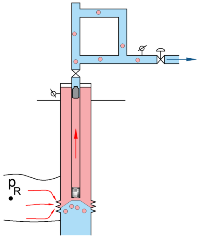
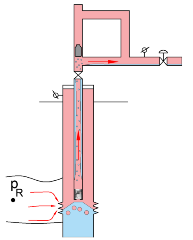
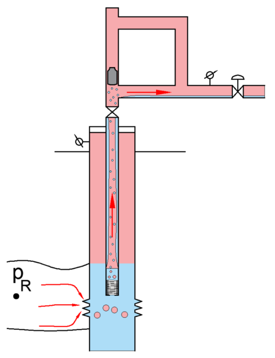
1.3.4. Static (Quiet) Side
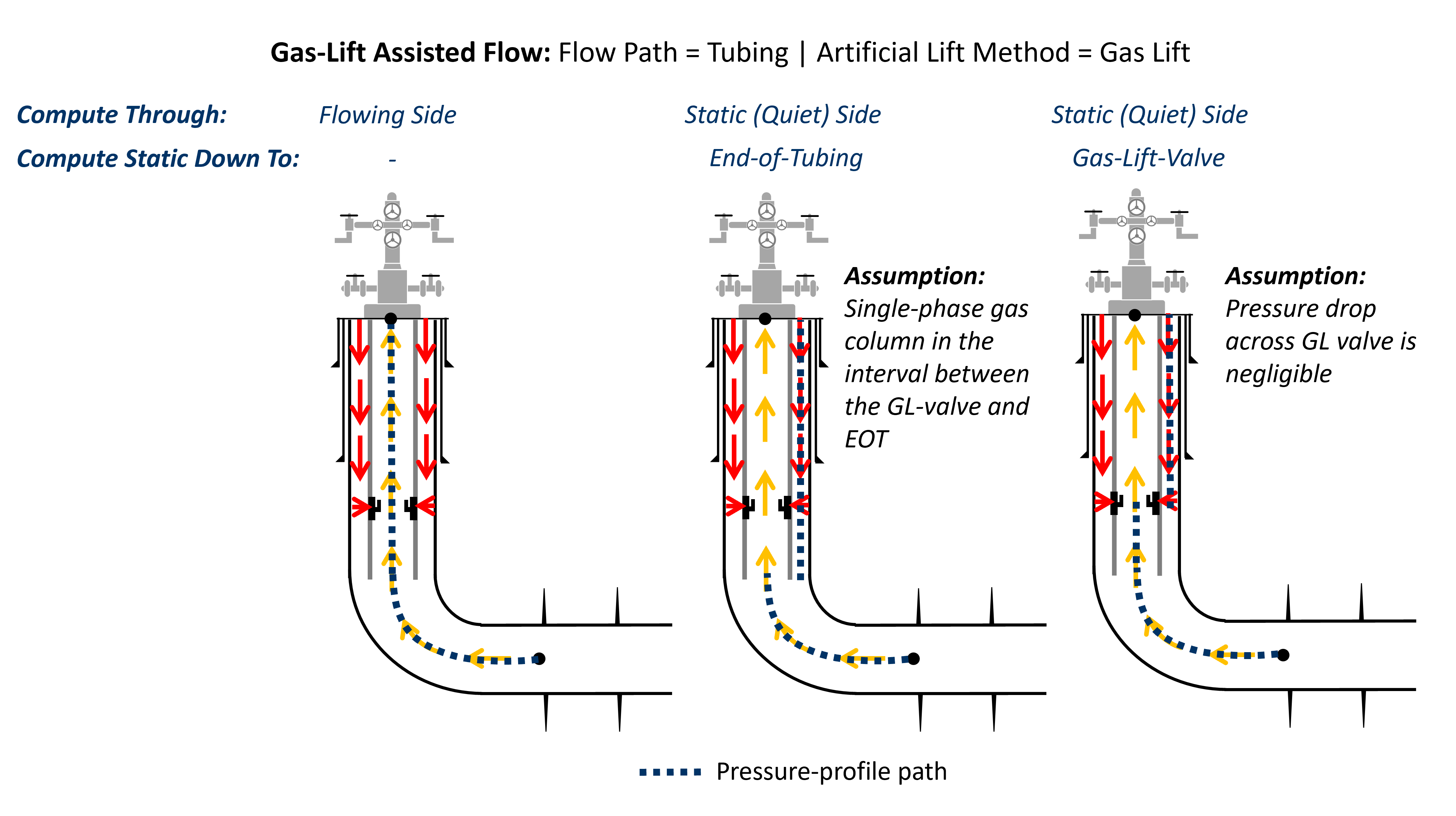
The user may select which side of the tubing the bottomhole-pressure calculation should follow. Using the static (quiet) side of the tubing assumes that there is a single-phase gas column with communication to the flowing side at the EOT (i.e., no isolating packer).
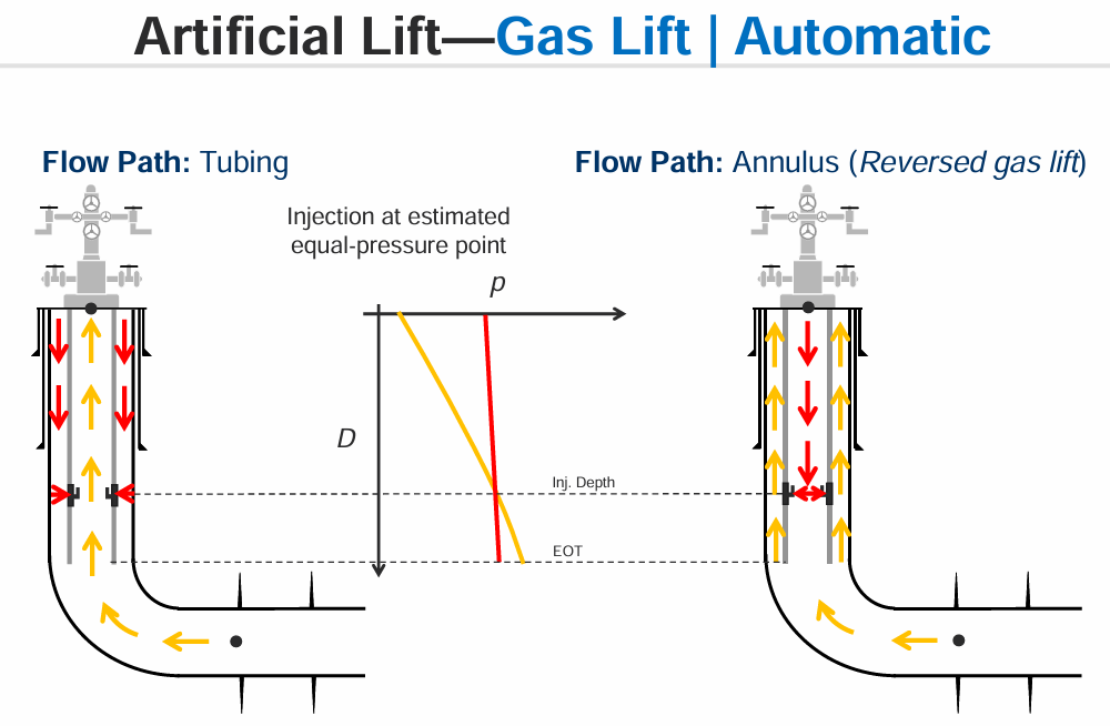
The static-side calculation is well suited for gas-lift assisted wells where it is certain that the static side is filled with gas at least down to the gas-lift valve. The figures below explain how the static-side calculation works for a naturally flowing well, and a gas-lift assisted well. The flow path in this case is set to "tubing", but the static-side calculation also works when the flow path is set to "annulus", with everything being reversed compared to the figures below.
For gas-lift assisted wells where the gas-lift configuration is set to "valves" or "automatic", it is also possible to select whether to do the static-side calculation down to the gas-lift valve or to the end of the tubing.
1.3.5. Convert from Gauge Pressure to Sandface
If the user has entered pressures for one or several rows in the Gauge Pressure column in production data, one can convert this pressure down to sandface. To do this, toggle on "Calculate from gauge to sandface using measured pressures".
When the "Calculate from gauge to sandface using measured pressures" switch is activated, the behavior of the software depends on whether a gauge depth is provided.
| Condition | Software Behavior for BHP Calculation |
|---|---|
| If a gauge depth is provided | The software will correct the gauge pressure from that gauge depth to the top perforation depth. |
| If a gauge depth is not provided | The software will continue calculating the BHPs as if the switch was not activated. |
For the switch to be useful, ensure that you have provided the gauge depth within the corresponding wellbore configuration.
1.4. Temperature Data
The temperature data require two inputs, the rock temperature at the surface and the average wellhead temperature for the production time series.
Flowing fluid temperature at a given measured depth is calculated (starting from bottomhole) by using an explicit form of the energy equation (piecewise exponential; see below, with more details in our wiki). The explicit form of the energy equation is derived assuming enthalpy difference can be expressed as , where is specific fluid heat capacity at constant pressure and is the temperature difference between fluid and formation.
This equation requires formation temperature at a given depth. This is calculated using a linear interpolation in TVD between the provided surface rock temperature and reservoir temperature. The equation also requires the ratio () of the overall heat transfer coefficient () and (), which is a priori unknown. The value of is found by iteration until the calculated wellhead temperature matches the user-provided temperature. This is done for every data point input to BHP.
1.5. Water & Lift-gas Properties
This section allows you to customize the properties of water and injected lift gas used in well calculations.
-
Lift-gas PVT:
By default, the Lift-Gas PVT option is set to Surface Gas SG, which automatically uses the specific gravity of the produced gas to represent the gas being injected for lift. This is a common assumption when the lift gas is recycled from the same well. Alternatively, selecting Specified SG allows you to manually input a different gas specific gravity if the lift gas comes from a different source. -
Water PVT:
You can also adjust the water salinity and water specific gravity. Editing one will automatically update the other, ensuring consistency in the water PVT properties used throughout your modeling. These settings directly affect the water density and viscosity and are calculated automatically.
1.6. Artificial-Lift Data
The BHP can be calculated while the well is on gas-lift, rod pump, plunger lift, or ESP.
| Artificial Lift Method | Activation Condition for a Given Day |
|---|---|
| None | The active wellbore configuration for that day has artificial lift set to None. No additional data is required. Natural flow assumptions apply. |
| Jet Pump | The active wellbore configuration for that day has jet pump as the artificial lift method, AND at least one of the following is provided in production data: Power Fluid Pressure or Power Fluid Rate (if both are provided, both are used). |
| Gas Lift | The active wellbore configuration for that day has gas lift as the artificial lift method, AND \(q_{g,\text{gas lift}}\) in the production data is greater than zero. |
| ESP (Electric Submersible Pump) | Can be activated only if downhole pressures are measured at the ESP inlet with a pressure gauge, and the gauge depth is defined. Pressures are corrected from the gauge to sandface. |
| Rod Pump | The active wellbore configuration for that day has rod pump as the artificial lift method, AND the Liquid Level in the production data is greater than zero. |
| Plunger Lift (GAPL, PAGL) | The active wellbore configuration for that day has plunger lift as the artificial lift method. If plunger-operating data exists, it is used; otherwise the method is considered active based on configuration. |
2. Output
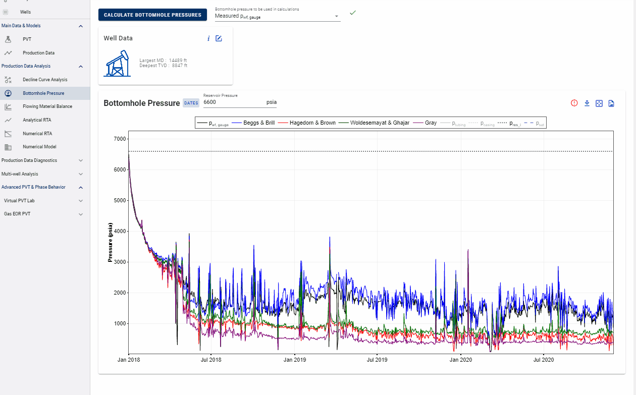
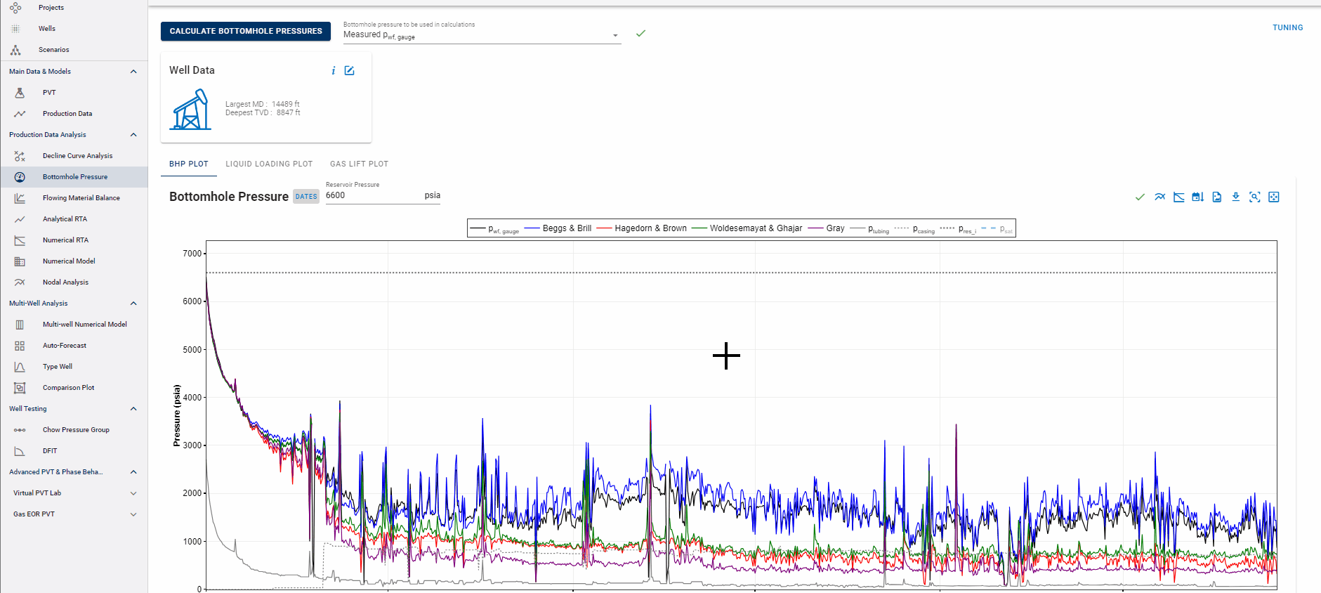
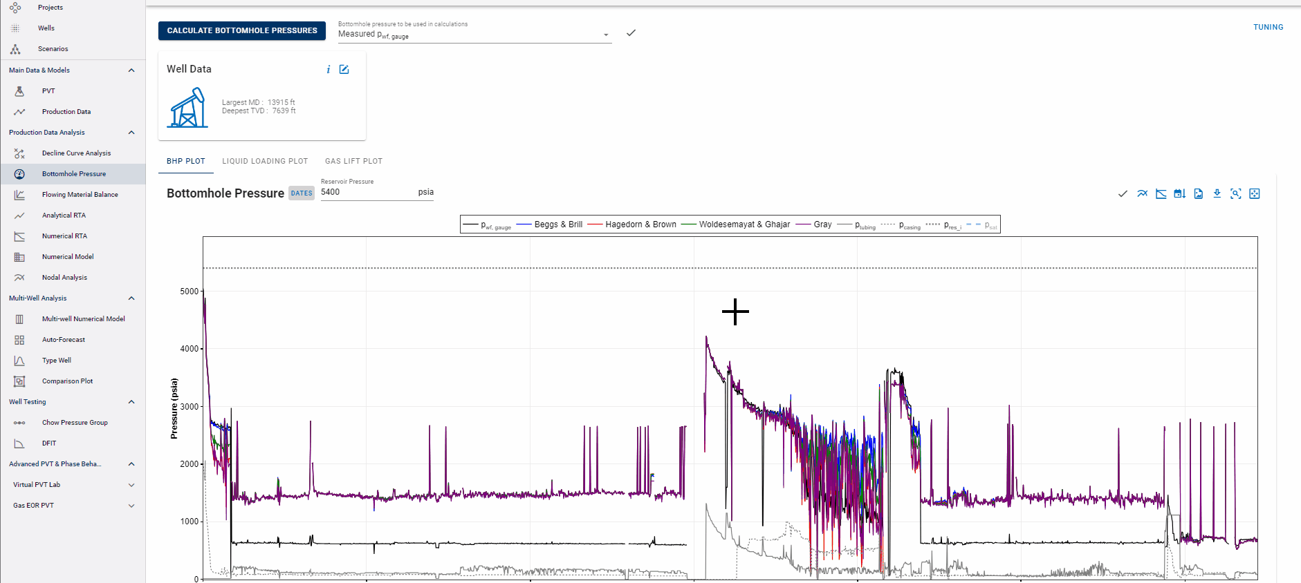
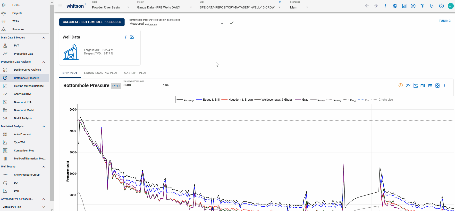
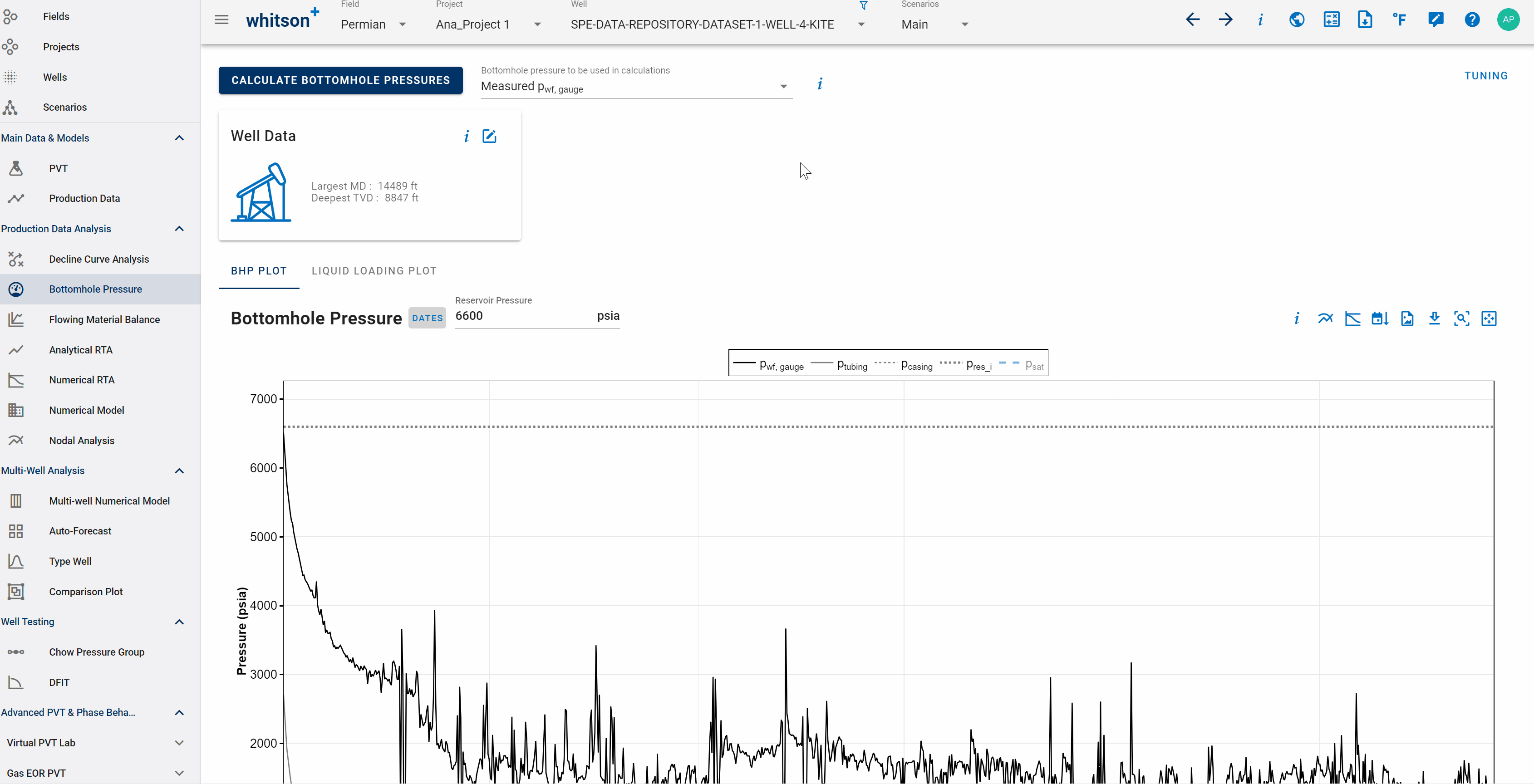
2.1. Output Curves
The output data for the BHP module is the calculated bottomhole pressure, at the top perforation depth, for every entry in the production time series. The user can choose whether to use the noisy data resulting from raw production data, or to apply a smoothing of the data. Furthermore, the user can select which BHP data set to use in other features of whitson+ that rely on bottomhole pressures. This ensures consistency in all calculations across the platform.
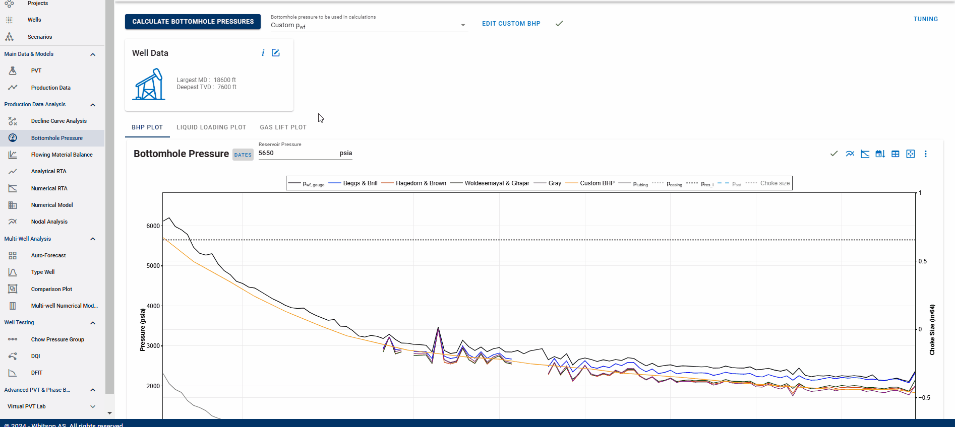
2.2. Custom BHP
Calculated bottomhole pressures are generally noisy due to oscillations in surface rates and pressures. This noise can significantly impact analysis, especially in RTA or numerical modeling when the well is controlled by bottomhole pressure. The Custom BHP feature allows users to smooth and piecewise-linearize the calculated bottomhole pressures. Users can define the sampling frequency, manually add or remove points to shape the desired BHP curve, and toggle an option to ignore zero-pressure values during the calculation. Additionally, an autofit line can be generated to assist with quickly establishing a baseline BHP profile.
2.3. BHP Calculation Stuck?
When the computation takes longer than expected, the user can try to force re-running the calculation as follows:
- Open Well Data card.
- Click Calculation Options.
- Click refresh icon to Force Run BHP Calculation.
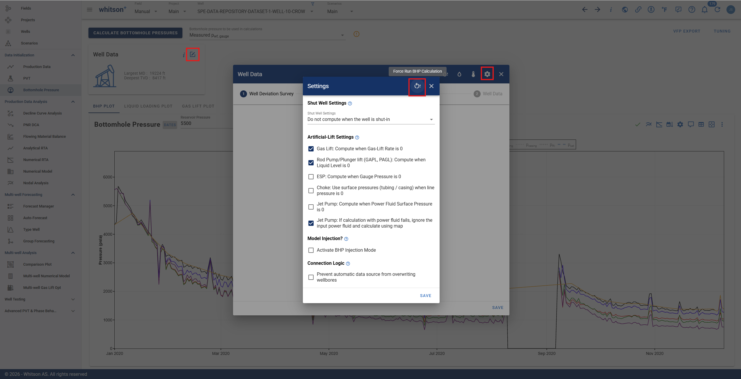
If the problem persists, please contact support@whitson.com.
2.4. BHP Plot Options
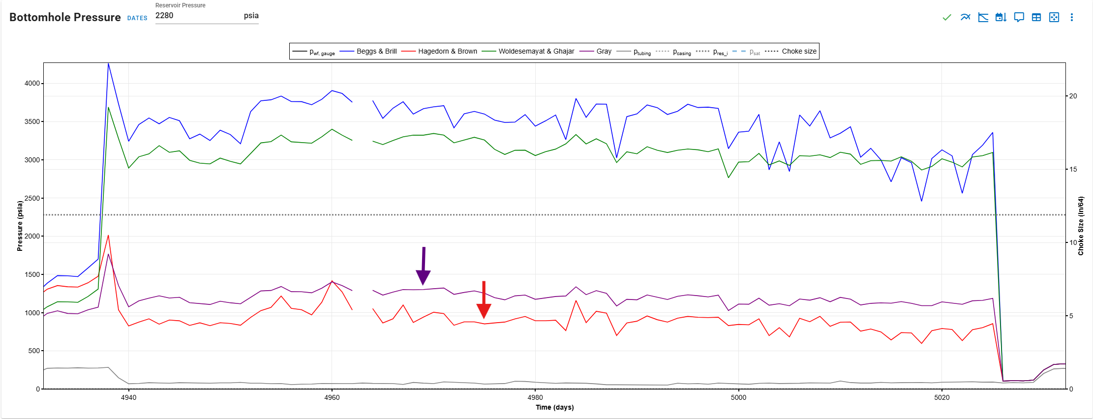
2.4.1. Show Rates, Surface Pressures
On the BHP Plot tab, you can plot the rates, as well as the surface pressures, alongside the bottomhole pressure calculation results.
2.4.2. Show Wellbore Configuration Dates
On the BHP Plot tab, you can visually examine how the wellbore configuration changes alongside the bottomhole pressure calculation results.
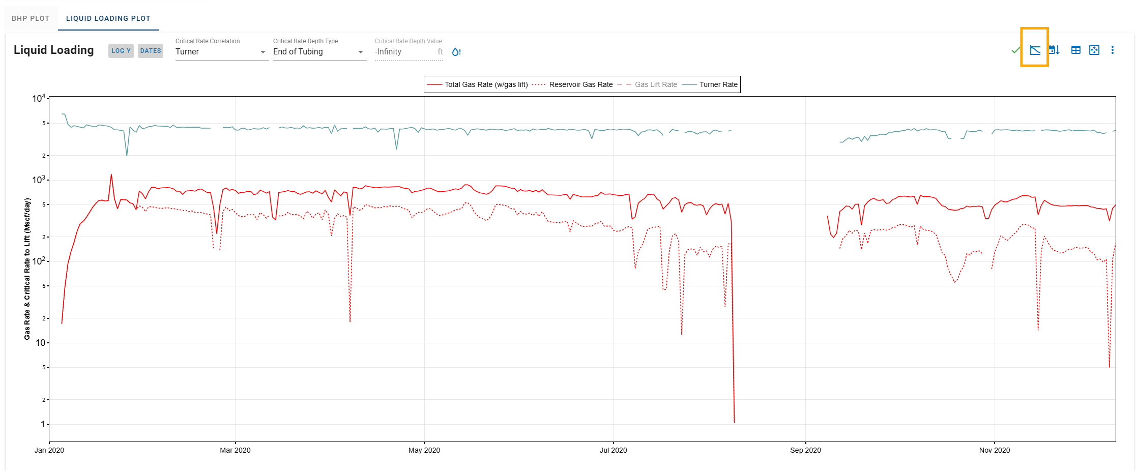
2.4.3. Show Liquid Loading
On the Liquid Loading Plot tab, you can compare your actual gas rates to the required critical gas rates to deliver gas through the current wellbore configuration without any liquid loading issues. See the Liquid Loading section for more details.
The critical rate is computed at the end of tubing using the Turner correlation by default. You can always change the correlation to use and the depth at which these critical rates are reported.
2.4.4. Show Gas Lift Injection Depth
On the Gas Lift Plot tab, you can see the depth of the valve at which the gas was injected and compare it with the casing, tubing pressure and the gas lift gas rate.
2.4.5. What Happens with Low Rates in the BHP Calculation?
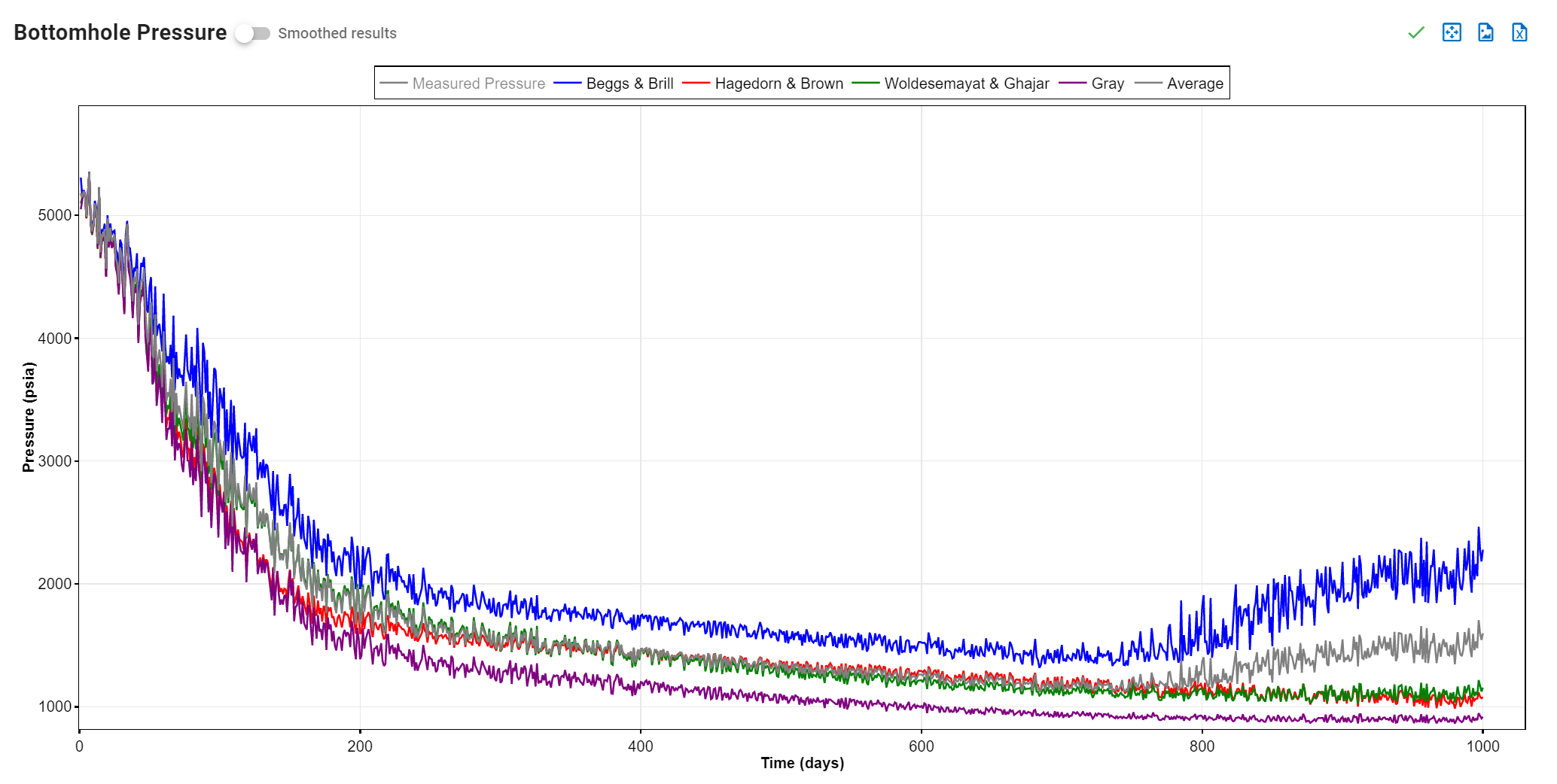
When the total production rate is relatively low and the liquid cut is high, the calculated BHP may vary significantly across the different correlations. In most cases, certain correlations may even return a BHP estimate higher than the initial reservoir pressure, which is clearly unphysical. Why does this happen?
It lies in the fundamental assumptions behind the pressure-drop correlations:
- Steady-state flow assumption – most correlations assume that flow in the wellbore is steady and continuous. GOR and WGR are assumed as constant throughout the well's history.
- Reality at low rates – at very low rates with high liquid loading, the well rarely flows steadily. Instead, unstable regimes such as slugging (large alternating gas and liquid slugs) or other unsteady-state behaviors are common.
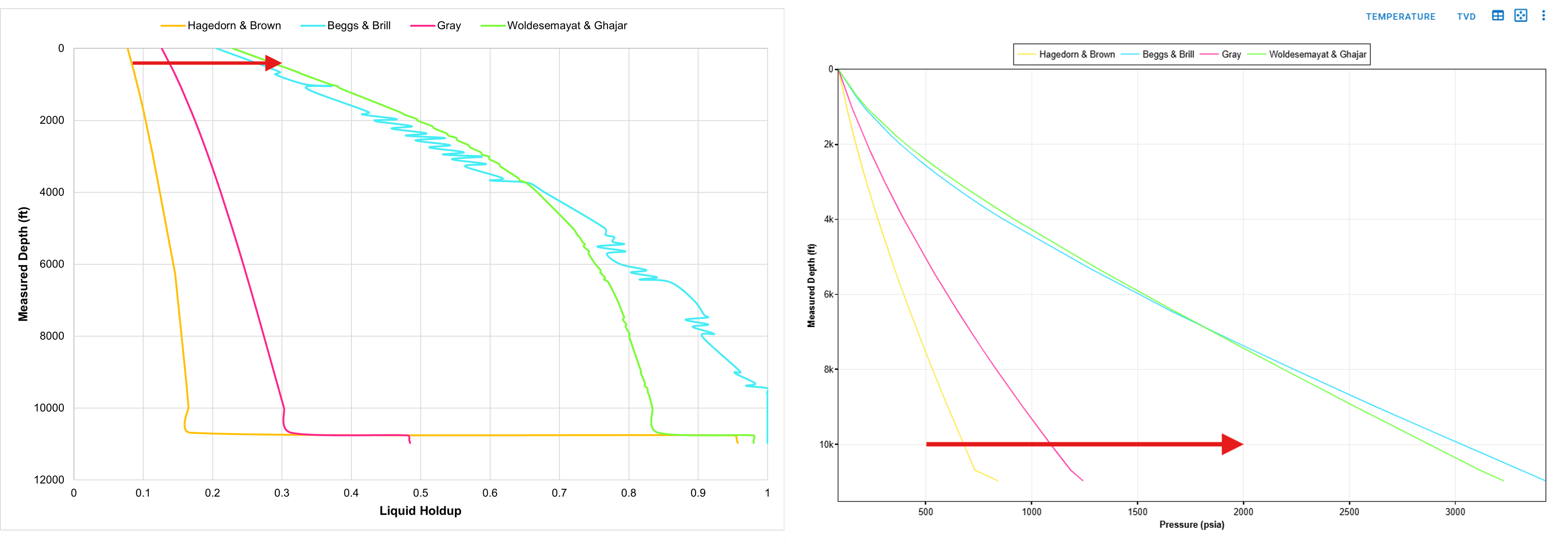
These unstable flow conditions strongly affect the estimated liquid holdup (), which is the key parameter in the pressure-drop equation:
where the effective density is:
Because estimates vary widely between correlations under these conditions, the resulting BHP calculations can also differ significantly.
Practical implications
This variability is exactly why we always calculate BHP using 4 correlations simultaneously.
- Large spread = warning sign for users – if the calculated BHPs diverge significantly, it is an indication that the calculation is less reliable. In such cases, the results should be interpreted with caution.
- Physical constraints – a correlation that produces BHP values higher than the reservoir pressure is unphysical and should not be used as the basis for decisions.
As illustrated in the figure below, even at the starting point of the calculation (surface depth), there can already be a significant difference in the estimated liquid holdup () between correlations. This difference propagates down the wellbore, resulting in diverging BHP estimates at the top of perforations (TOP).
Selecting a BHP correlation at low rates
In low-rate, high-liquid situations, use the correlation that provides the most physically realistic estimate (i.e., lower than the reservoir pressure). However, remember that none of the standard correlations are fully predictive under unstable flow regimes. Treat the results as approximate indicators rather than precise values.
3. Technical Features
3.1. Governing Equations
The main equations used for multiphase flow in inclined pipe are provided here. Our wiki contains a detailed review of the relevant multiphase-flow theory and the commonly used correlations for pipe flow.
3.2. Artificial-Lift Methods
3.2.1. Gas Lift
Gas lift is included as a step change in mass flow at the injection valve. We assume the lift gas to completely mix with the flowing mixture, resulting in a step change in the gas rate, and consequently the producing GOR.
When the well is on gas lift, are gas rates netted or gross (including gas lift rates)?
The gas rates entered in the production data editor are assumed to be netted out
The reason we do this is because the gas rate is used everywhere in the system, including numerical model, flowing material balance and RTA; and there the gas lift is not part of the calculation (i.e. not part of the reservoir flow).
In the BHP calculations, to get the total gas that is flowing inside the wellbore, we just do the calculation in the background as follows:
Three options exist for the gas-lift configuration:
1. Poorboy: The term "poorboy" refers to the situation when injection occurs at the EOT.
2. Valves: A single valve at a specified depth, or a set of valves at different depths along the tubing, can be provided. If a full set of valves is provided, the casinghead pressure is used to decide which valve the lift-gas enters the tubing through. We assume all of the lift gas to enter the tubing through the first open valve it encounters, even though this rate might exceed the maximum rate predicted by the Thornhill-Craver equation.
Gas Lift Valve Ordering and Behavior
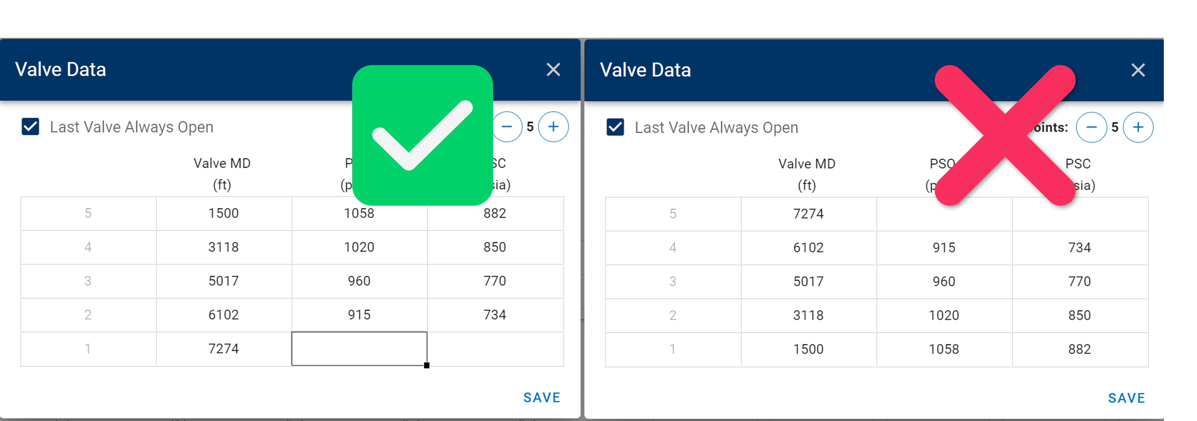
The gas lift valves are ordered by descending measured depth with valve number. The deepest valve is valve number 1, the second deepest is valve number 2, and so on. If "Last Valve Always Open" is ticked, then PSC and PSO for valve 1 (if specified) will be disregarded by the calculator.
3. Automatic: If the lift-gas injection depth is unknown, then the BHP calculator can estimate the depth by computing the pressure profiles in the tubing and annulus and finding the depth at which they are equal. If this depth is computed deeper than the EOT depth, then EOT depth is used (poorboy).
If the flow path for a given day is set to "Annulus", a reversed gas-lift configuration is applied where the point of injection is set to be at the deepest valve if there is only a single valve depth specified or "Last Valve Always Open" is ticked for a set of valves. If not, the lift-gas is injected at the EOT.
Which gas lift configuration should I choose for a given well?
Is there a packer in the well? If so, the gas lift configuration likely uses valves, meaning the injected gas enters through gas lift valves in the tubing. In this case, the depth of the valve(s) that allow gas to flow from annulus to tubing, or vice versa, is a required input.
If packers are installed but the valve depth is unknown, then selecting the Automatic gas lift configuration is usually the best choice. The BHP calculator can estimate the injection depth by computing the pressure profiles in the tubing and annulus and finding the depth where they are equal. One important consideration is that using the Automatic gas lift configuration may result in injection occurring at the end of tubing (EOT), which would not be consistent with having a packer in the hole. However, this only occurs if the computed injection depth is deeper than the EOT based on the input data.
If there is no packer installed, there is communication between the annulus and tubing through the end of tubing (EOT). Therefore, the appropriate gas lift configuration is usually Poorboy.
Differences in Gas Lift Configurations
-
Gas Lift configuration "Valves" are assumed to open in the direction Annulus → Tubing (conventional logic). This means that when lift gas is injected into the annulus (i.e., flowpath = Tubing), the gas will enter the first valve that opens based on the casinghead pressure (CHP).
-
If lift gas is instead injected into the tubing (i.e., flowpath = Annulus), the gas will typically travel down to the end of tubing (EOT) and enter the well stream directly—this setup is referred to as a "poorboy" configuration.
-
If the "Last Valve Always Open" option is checked, the gas can bypass the poorboy path and flow through the last valve, which is assumed to always be open. Gas lift valves are one-way valves, allowing flow only from annulus to tubing. The exception is the last (deepest) valve, which can be treated as a simple orifice (an open hole) if the "Last Valve Always Open" setting is enabled.
-
Gas Lift configuration "Reversed Valves" results in the opposite logic, with all valves opening in the direction Tubing → Annulus.
| Flowpath | Gas Lift Configuration | Lift Gas is Injected Into | Lift Gas enters well stream at |
|---|---|---|---|
| Tubing | Poorboy | Annulus | EOT |
| Annulus | Poorboy | Tubing | EOT |
| Tubing | Valves | Annulus | First Open Valve |
| Annulus | Valves | Tubing | Last Valve if "Last Valve Always Open", else EOT |
| Tubing | Reversed Valves | Annulus | Last Valve if "Last Valve Always Open", else EOT |
| Annulus | Reversed Valves | Tubing | First Open Valve |
When using "Unknown" flowpath, the Gas Lift Valve direction is important. This is because the same gas lift well configuration can be used while swapping the flow path between Tubing and Annulus by the maximum wellhead pressure between CHP and THP.
3.2.1.1. Single Point High Pressure Gas Lift (HPGL)
Single-point high-pressure gas lift refers to the situation in which high-pressure gas is available and one can get to injection depth without using unloading valves. In this case, the tubing has a single lift gas injection point. Sometimes, no gas lift valves are used; lift gas is injected at EOT, which also allows the injection point to reach deeper into the lateral.
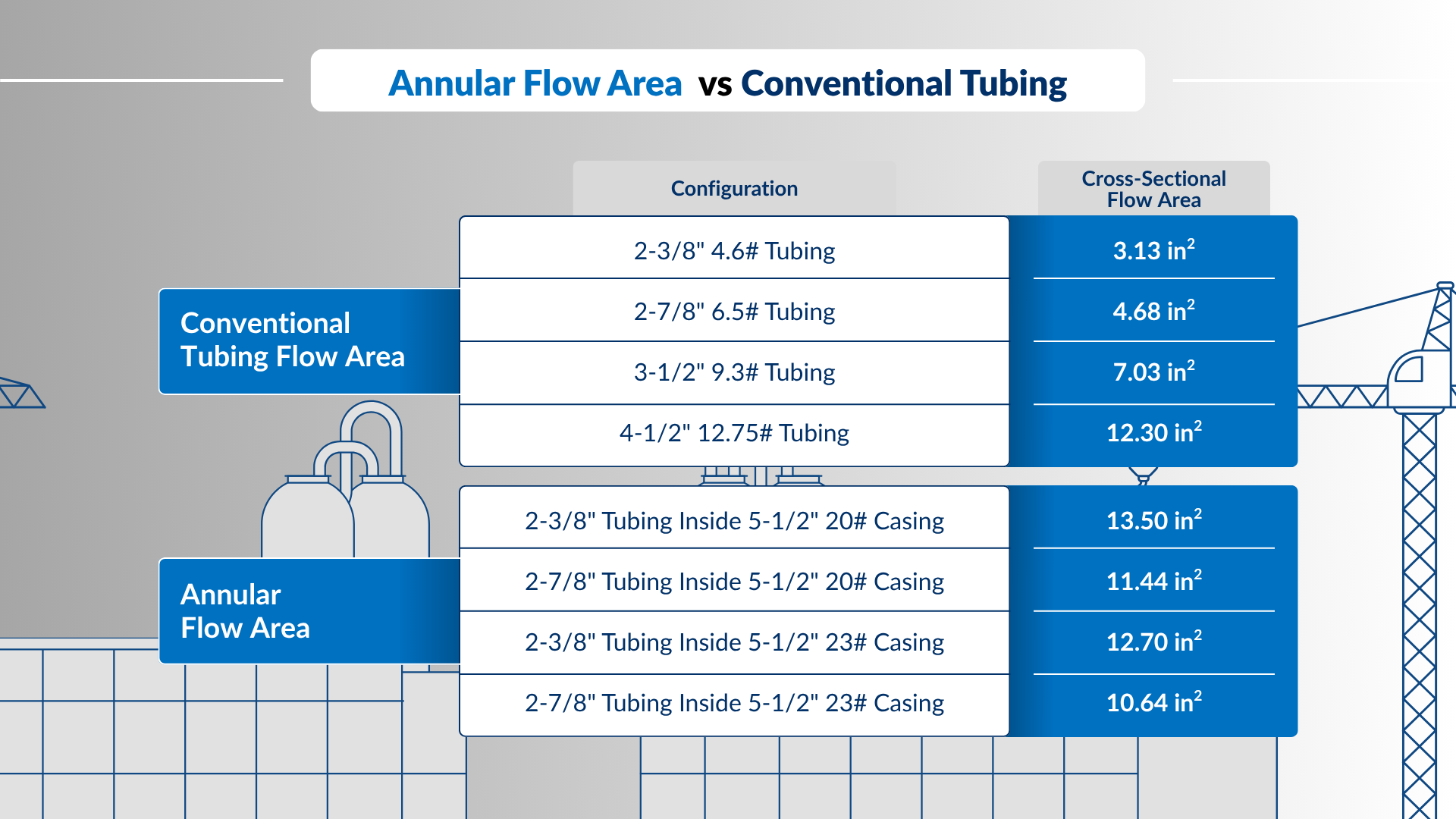
A design choice that is sometimes used for HPGL is to use inverse gas lift (lift gas is injected through tubing and fluids produced through annulus). This gives a bigger flow area, which allows high reservoir rates to be transported without excessive pressure drops. The table below shows a comparison between the cross-sectional flow area when using tubing or annular configuration for different tubing and casing sizes. For example, if one flows through the annulus of a 2-3/8" tubing inside a 5-1/2" 23# casing, it is equivalent to flowing through a 4-1/2" 12.75# tubing.
To model HPGL, just provide a single valve (or select Poorboy if using EOT injection) and select annulus as flow path if gas lift is injected through tubing.
3.2.2. Rod Pump
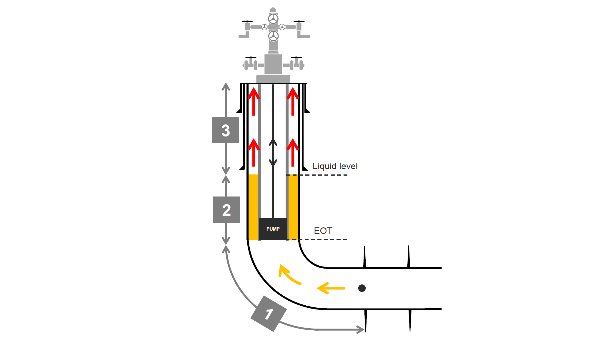
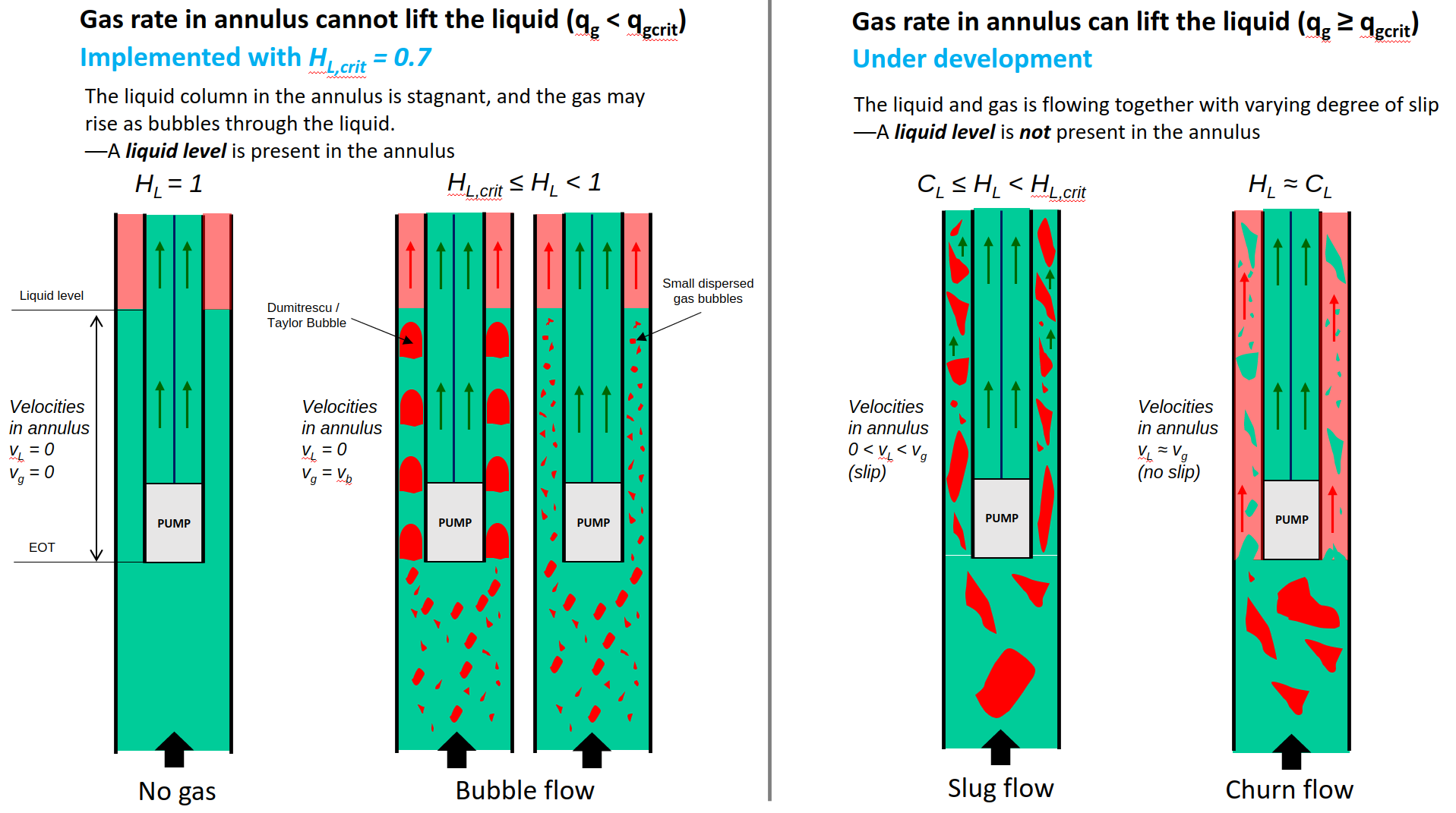
BHP calculations with a rod pump are achieved by dividing the well into three parts:
-
Top Perforation to Inlet of Pump (EOT)—Full well stream flowing in production casing, regular multiphase pipe flow.
- BHP is calculated using the correlation specified.
-
Inlet of Pump (EOT) to Liquid Level in Annulus—Static liquid column with gas bubbles percolating through it.
- This section does not use any correlation; instead, the logic is based on calculating the bubble velocity of a Taylor bubble and small bubble.
- The smaller velocity is assumed to be the slip velocity, which is then used to calculate HL. The liquid hold-up (HL) is limited to ≥ 0.7.
- An inclination correction is applied to the slip velocity.
-
Liquid Level in Annulus to Wellhead—Single-phase gas flow in the annulus. Gas percolating through the liquid column flows to the wellhead.
- This section is calculated as single-phase gas flow, meaning correlation selection has no impact.
Which part is affected by correlation selection?
The selected correlation affects the BHP calculation only in Section 1 (Top Perforation to EOT).
We assume the fluid split at the inlet of the pump to be such that all surface gas goes through the annulus, and all liquid goes through the pump and up the tubing. This is an approximation of the true split, and thus the estimated BHP may be somewhat larger than the true solution (less gas goes through the annulus in real life than what is modeled).
Most of the pressure drop for rod pump occurs in the second part, (i.e., the static column of fluid) as this is most-often along the vertical part of the well where the gravity pressure drop dominates. This fluid column will in most cases be liquid-like where the liquid is stagnant and the produced gas is percolating/rising through the liquid as bubbles. A new model to honor this liquid-like fluid column has been introduced to the rod-pump calculations, as the original model was overly sensitive to gas rate and consequently predicted too low pressure drop in the fluid column.
Why can't I select between flowing side or static (quiet) side when artificial lift is set to rod pump?
Casing pressures are always used as a pressure source for rod pumps, ignoring tubing pressures. Therefore, it is always a static (quiet) side calculation, and hence there is no option to choose between flowing and static (quiet) side.
The figure below shows four flow regimes/modes for rod pump.
-
The flow regimes to the left represent the situation when the gas is not able to carry the liquid with it, causing a well-defined liquid level in the annulus. This model has been implemented, with a critical liquid hold-up set to 0.7.
-
The flow regimes on the right represent the situation when the gas is able to carry liquid with it. This is not implemented yet.
Unifying the left and right flow modes requires (1) a method of estimating the critical liquid hold-up (i.e., the transition between left and right models), and (2) a method of estimating the fraction of the total produced liquids that goes up the annulus. This is under development.
3.2.2.1 Liquid Level for Rod Pumps
Liquid level measured depths (MD) are required for rod pump configuration. If no liquid level is provided in the production data (or it is set to zero), BHP calculations will not be performed.
You can change this behavior by editing the well configuration and enabling the option to compute when liquid level is zero or empty as shown below.
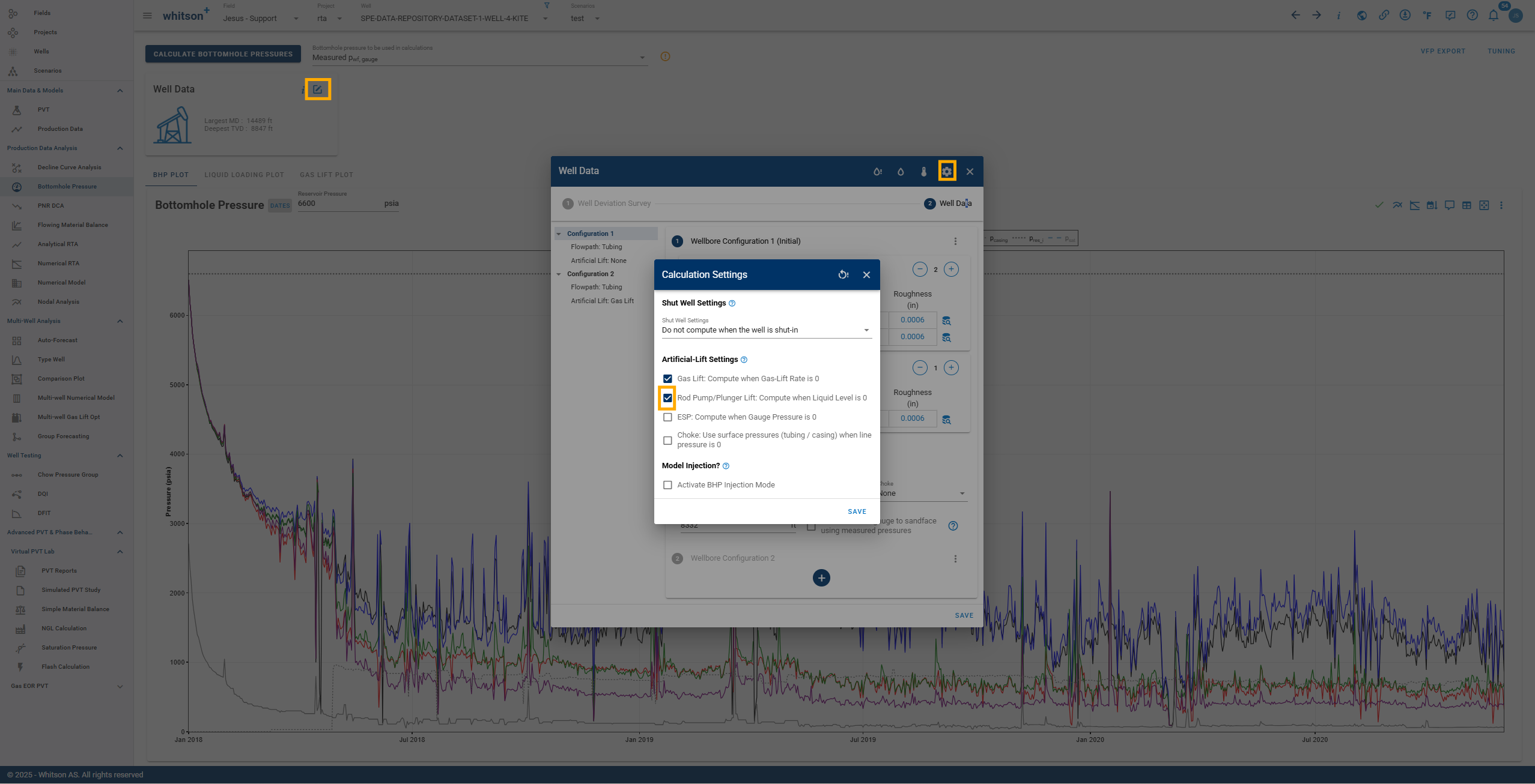
This setting will assume no pump is present in the well and will calculate under natural flow conditions. As a result, the calculated BHP values will often be much higher than actual, since a pump typically reduces BHP.
If you want to assume an annulus column filled with gas, set the liquid level measured depth to the end-of-tubing (EOT) depth or pump depth in the production data.
Difference in BHP values
Be aware that liquid and gas columns produce significantly different BHP values because of the density difference; this means BHP values calculated with a liquid level will be larger than those calculated assuming a gas column.
3.2.3. Plunger Lift
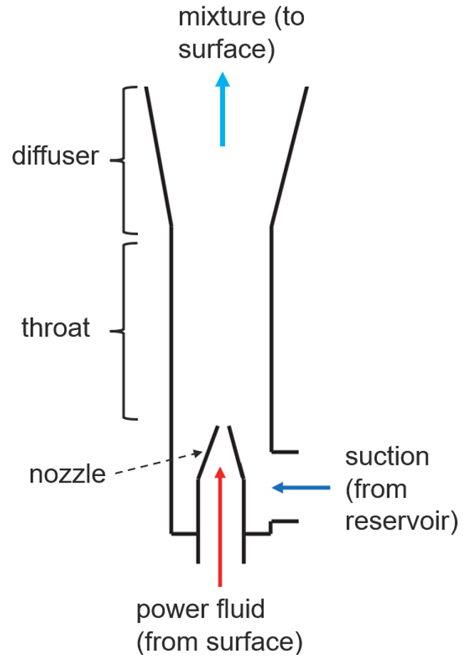
Plunger lift is a deliquification method used to remove liquids accumulated at the bottom of the well and improve production. It is often used to counteract liquid loading issues in gas wells. A schematic of a plunger lift system is shown in the figure below.
where, the gray component in the figure represents the plunger, which is essentially a cylindrical piston that travels up and down inside the tubing. The plunger's actuation is controlled by the opening and closing of the motorized valve at the surface.
- Upward travel: the piston lifts accumulated liquids from the bottom of the well, reducing flowing bottomhole pressure and improving production.
- Downward travel: when liquid accumulates again, the well is shut-in, allowing the piston to descend before the cycle repeats.
Plunger lift stages:
Stages 1-2, well shut-in ("off" time). The well is shut in using the motorized valve, gas production at the surface and in the tubing is interrupted. Liquids slide down and accumulate at the bottom. The plunger drops and travels downward through tubing until it stops at a bumper spring at the bottom. The plunger typically moves at 5 m/s or less, so it might take some 20-40 minutes to reach the bottom. The bottomhole pressure (BHP) increases due to reservoir influx, while gas is stored in the annulus, preparing for the next lift cycle. After the plunger lands, the well can be kept shut in for a few more minutes to allow BHP to build up further, enhancing liquid displacement and ensuring higher gas production rates when the well is reopened.
There are some plungers called "bypass" that have a hole through them. This allows the well to be shut in for only a few seconds/minutes for the plunger to start falling, and then the well is put back into production. Production fluids flow upwards through the plunger while the plunger falls down. When it reaches the bottom, the plunger bottom assembly closes the hole and then production fluids push it back up.
Stage 3, production start ("on" time). When the motorized valve is opened, the plunger is pushed upward by the gas stored in the near-wellbore region and casing. The plunger velocity typically is below 5 m/s, thus it might take the plunger 20-30 minutes to reach the surface. During this stage, gas above the liquid slug (pushed by the plunger) is produced, and some gas may bypass the plunger and liquid slug.
Stage 4, afterflow. The plunger reaches the top and it is parked. The gas flowing behind it is redirected through a bypass line, which is often accompanied by a modest increase in gas flow rate, as the gas no longer needs to push the plunger and liquid slug. The gas now flows through an unobstructed pipe, and the wellbore is free of liquids, allowing for more efficient production.
For the rest of stage 4, reservoir gas and liquid enter the wellbore. Most of the liquid remains behind, being accumulated at the bottom of the well. The duration of this stage is typically a few minutes or fraction of an hour since liquid fills the tubing quickly, but it depends on the liquid gas ratio of the well and size of tubing and casing.
- The cycle is repeated (back to stage 1).
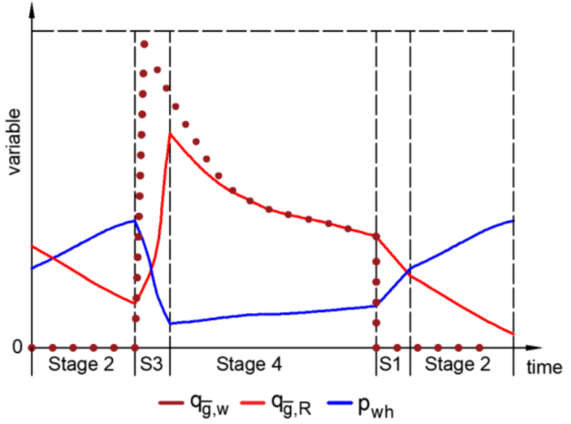
The figure below illustrates the evolution of key well parameters across the four plunger lift stages: gas rate in the tubing (dark red dots), reservoir influx (bright red line), bottomhole pressure (blue line), and flowing bottomhole pressure (solid green).
3.2.4. Gas-Assisted Plunger Lift (GAPL) and Plunger-Assisted Gas Lift (PAGL)
3.2.4.1. GAPL vs PAGL - What's the Difference?
Many people use these terms interchangeably to refer to combinations of gas-lift and plunger-lift. While we know of no formal SPE definition, we use GAPL to refer to gas-assisted plunger-lift, and PAGL to refer to plunger-assisted gas-lift. Both methods usually require a bottom-packer and gas is injected through the annulus below the bottom plunger assembly.
| Combination Lift Type | Description |
|---|---|
| PAGL (Plunger-Assisted Gas Lift) | Continuous gas-lift supported by a continuous-run plunger (bypass). |
| GAPL (Gas-Assisted Plunger Lift) | Conventional plunger (no bypass) supported by intermittent gas injection (no injection during shut-in). |
3.2.4.2. How to Calculate BHPs for Plunger-Lifted Wells or GAPL/PAGL Systems?
When a well is operating on plunger lift, the wellbore flow undergoes continuous short flow transients due to the cyclical nature of the plunger-lift process. Calculating bottomhole pressure under these conditions requires a small-time-scale simulation of the transient process. Such detailed simulations are beyond the typical scope of what we normally do for practical petroleum engineering applications. However, it is still possible to calculate an average steady-state bottomhole pressure for plunger-lifted wells as follows:
Option 1 (for wells with plunger lift only and no bottom packer): If liquid level is measured in the annulus, provide a liquid level together with the production data. Make sure the liquid levels input correspond to times when the well is producing. To use this calculation option, select "Plunger Lift (GAPL, PAGL)" as the artificial lift method, and select "Static (quiet) Side" in the "Compute Through" option. This method is similar to how BHP is calculated for rod pump wells when liquid levels are available.
Option 2 (for wells on plunger lift, GAPL, or PAGL): To use this calculation option, select "Plunger Lift (GAPL, PAGL)" as the artificial lift method, and select "Flowing Side" in the "Compute Through" option. In the well configuration, you must provide the following:
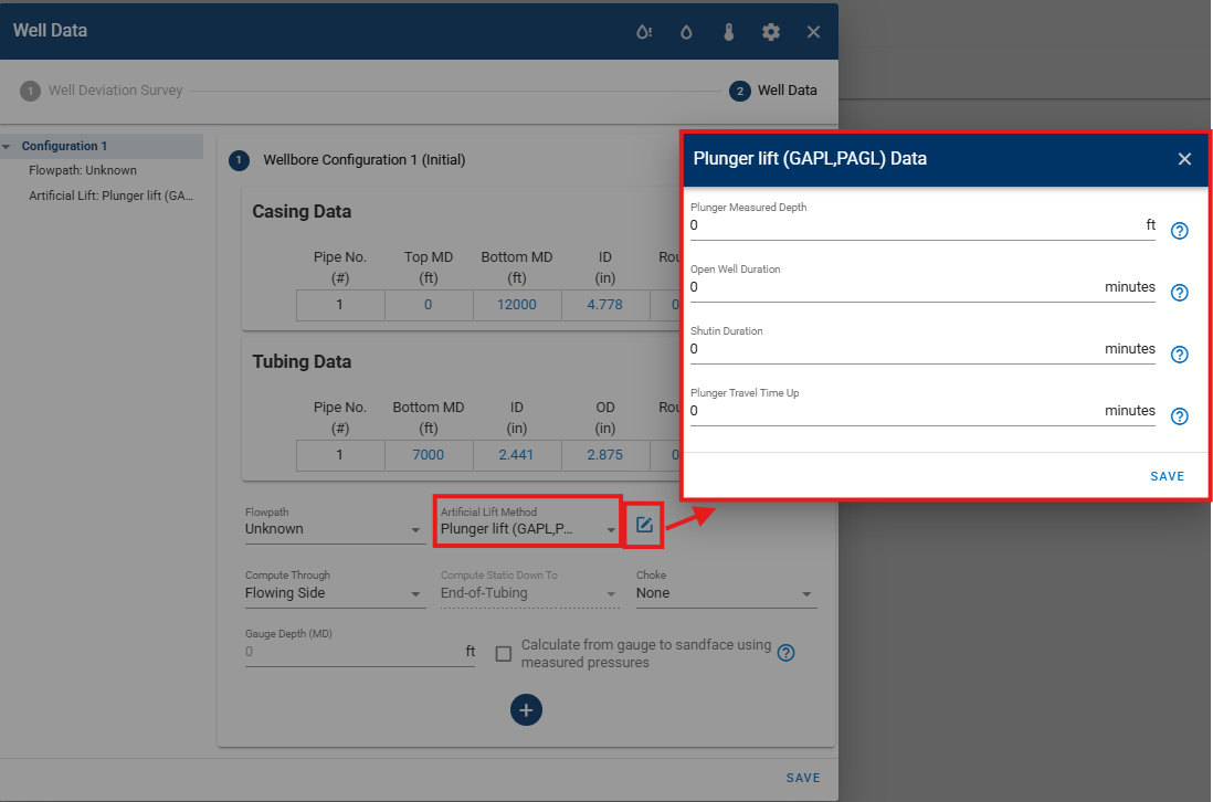
-
Depth of plunger lift bottom assembly (if there is gas injection, this is also the depth where the gas will be injected)
-
Duration of the open well cycle, in minutes
-
Duration of the shut-in cycle, in minutes
-
Plunger travel time up, in minutes
The standard rates of gas, oil, water and lift gas are modified to account for the fact that they are producing for a fraction of a day only, by multiplying them by the following factor:
Before applying this correction, input oil and water rates are reduced by the daily standard volumes transported by the plunger. The daily standard volumes transported by the plunger are found by running a BHP calculation with the original unmodified rates of oil, gas, lift gas, and water. From this calculation one obtains the holdup profile of oil and water along the wellbore. Then volumes are converted to standard conditions and integrated from the plunger bottom assembly to wellhead. The resulting standard oil and water volumes are then multiplied by the number of trips the plunger performs in a day:
Plunger lift, PAGL, and GAPL cases will be handled depending on the user input. Plunger lift has a lift gas rate equal to zero and a long shut-in to allow for the plunger to travel downwards. PAGL has a very short shut-in, since the plunger is bypass, and a lift gas rate different than zero. GAPL has a longer shut-in, with a lift gas rate different than zero.
Liquid loading flag behavior for plunger-lifted wells
The liquid loading flag is based on comparing the well’s reservoir gas rate + lift gas rate against the minimum rate to lift liquids (Turner, Coleman, Nagoo, or Belfroid) at the selected depth (or across all depths if a gradient check is used).
For plunger-lifted wells, BHP calculations can be performed using either the Flowing Side or the Static (quiet) Side (liquid level):
- Flowing Side: liquid-loading checks can be evaluated at all tubing locations (all depths available for the check).
- Static (quiet) Side: liquid-loading checks are only evaluated at locations below EOT.
Even when a plunger is installed and operating correctly, the flag can still indicate loaded. During the production cycle, the gas rate can decline and there may be periods where it falls below the minimum lift rate, allowing liquids to start accumulating. This can occur under both Flowing Side and Static (quiet) Side calculation approaches, so “Loaded” may reflect transient accumulation during the cycle rather than a sustained operational failure to unload.
3.2.4.3. IPR and Nodal Analysis for Plunger-Lifted Wells or GAPL/PAGL Systems?
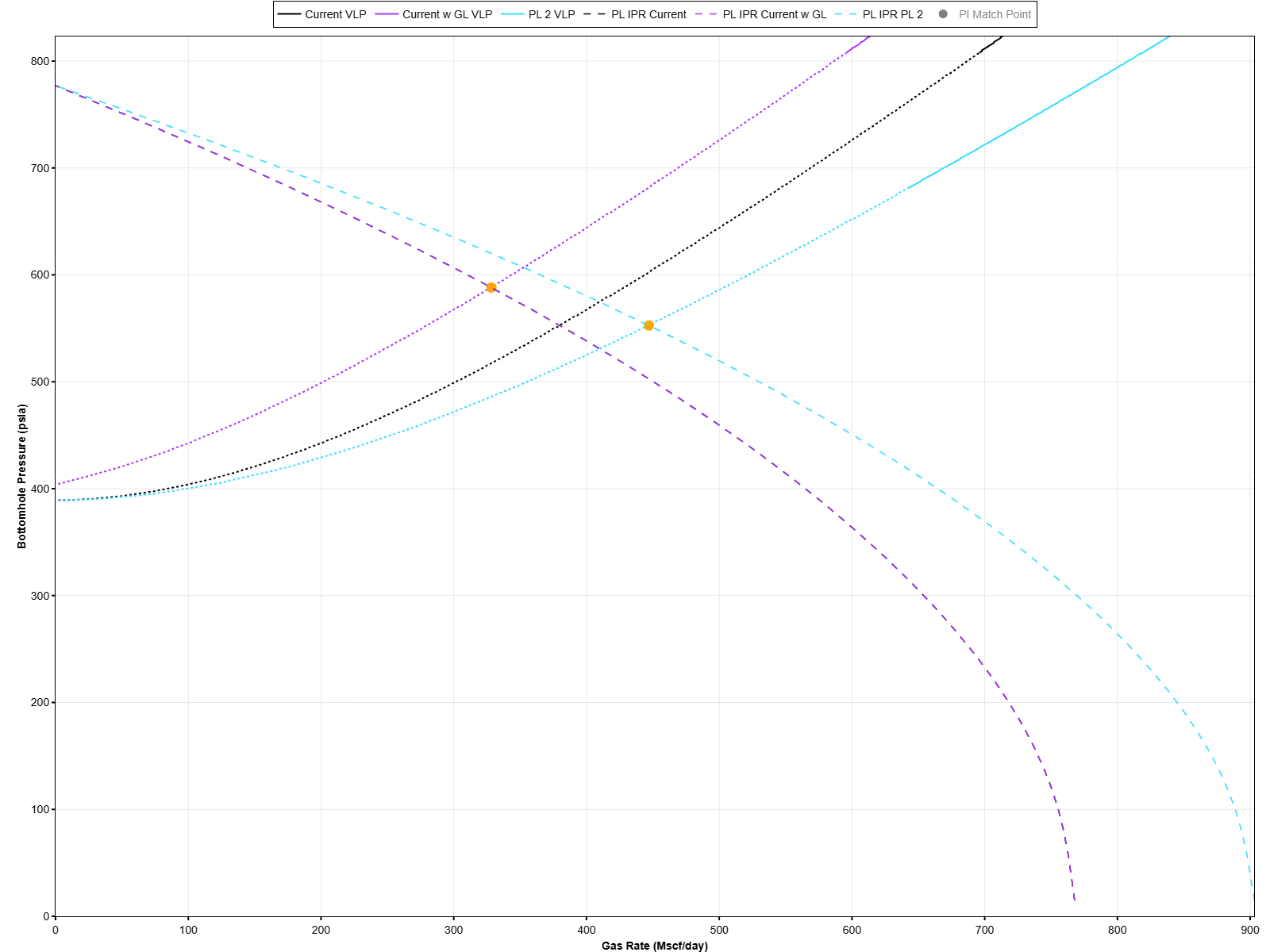
When the user first enters the IPR-VLP tool in the Nodal Analysis module, the IPR and VLP curves shown there (and the IPR parameters shown in the left side panel) are expressed in terms of daily rates. In consequence, the IPR is only valid for a specific combination of open and closed cycle durations. If the user changes those (for example when performing sensitivity studies to evaluate another plunger operational setup) a new IPR will be calculated.
As an example, consider the figure below that shows the IPR-VLP intersections for three cases: "Current" (a plunger lift configuration), "Current w GL" (a plunger lift configuration with gas lift) and "PL2" (a plunger lift configuration with different cycle durations).
Both "Current" and "Current w GL" cases share the same IPR, since the cycle durations are the same, but have different VLPs, since one considers lift gas while the other doesn't. Cases "Current" and "PL2" have different IPRs (and VLPs), since PL2 has slightly different cycle durations.
The IPR for a new combination of plunger lift cycle duration is calculated from the "real" IPR of the formation (calculated using the actual rates that occur during the production part of the plunger lift cycle). This "real" IPR will be displayed (and used for IPR-VLP intersections) if the user adds to the IPR-VLP case matrix a case without plunger lift (see the figure below, a case is added with natural flow, no artificial lift).
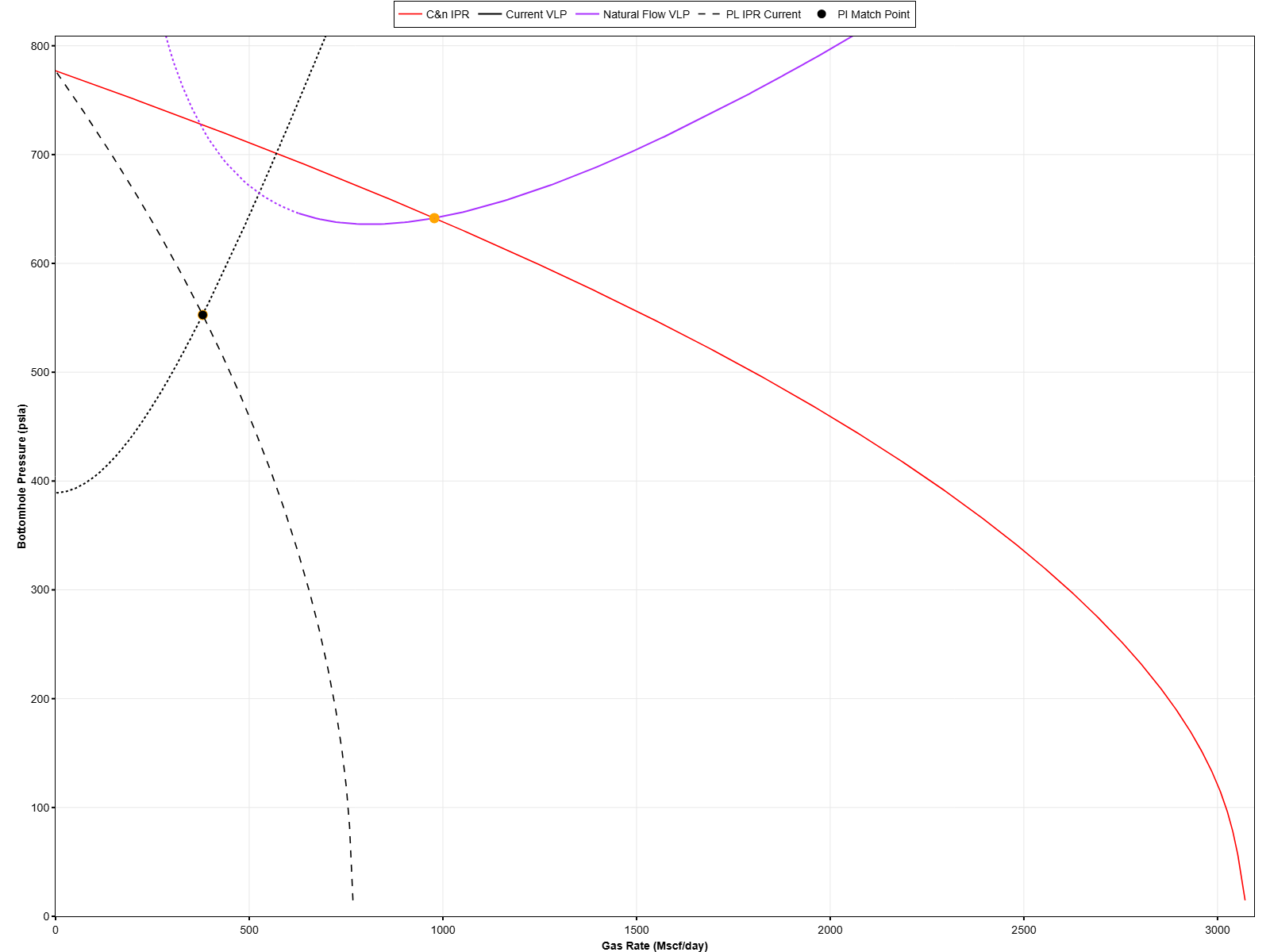
Plunger lift uses IPR C&n method only
Plunger lift uses the C&n method only for IPR estimation.
Limitations of IPR for plunger lift
The IPR methodology explained above assumes that there is a unique ("average") IPR during the complete plunger lift production cycle and that it can be expressed using equations developed for pseudo steady-state conditions. For some cases this might not be accurate, since, in practice, there is a formation transient triggered by well shut-in and opening, which could give higher productivities during the start of the cycle.
3.2.5. Jet Pump
3.2.5.1. Working principle
A jet pump typically has the following generic configuration:
This pump is typically installed as part of the tubing. Power fluid, usually dead oil or produced water, is injected through the nozzle, where it is accelerated. According to Bernoulli’s principle, this acceleration causes a pressure reduction, reaching a minimum at the nozzle tip. This minimum pressure generally provides a good approximation of the pump’s suction pressure.
Reservoir fluid enters through the annular region surrounding the nozzle. At the throat, the slow-moving reservoir fluid mixes with the fast-moving power fluid, which increases its velocity. The mixture is then slowed down in the diffuser, converting the kinetic energy into pressure.
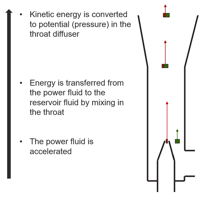
This is similar to what occurs in a centrifugal pump, except that in a centrifugal pump the acceleration is provided by the impeller, whereas in a jet pump, external fluid is used.
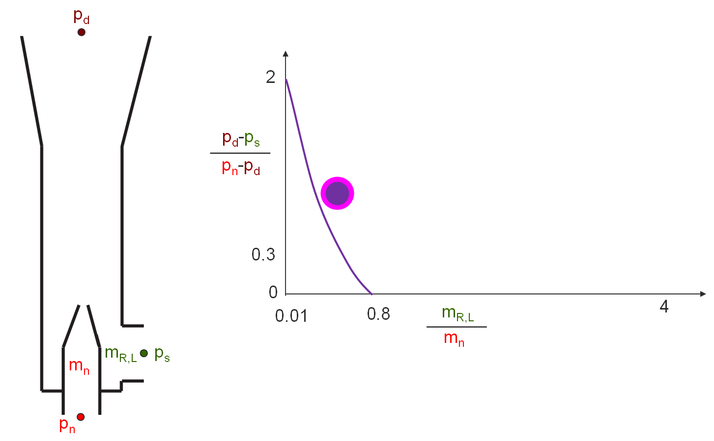
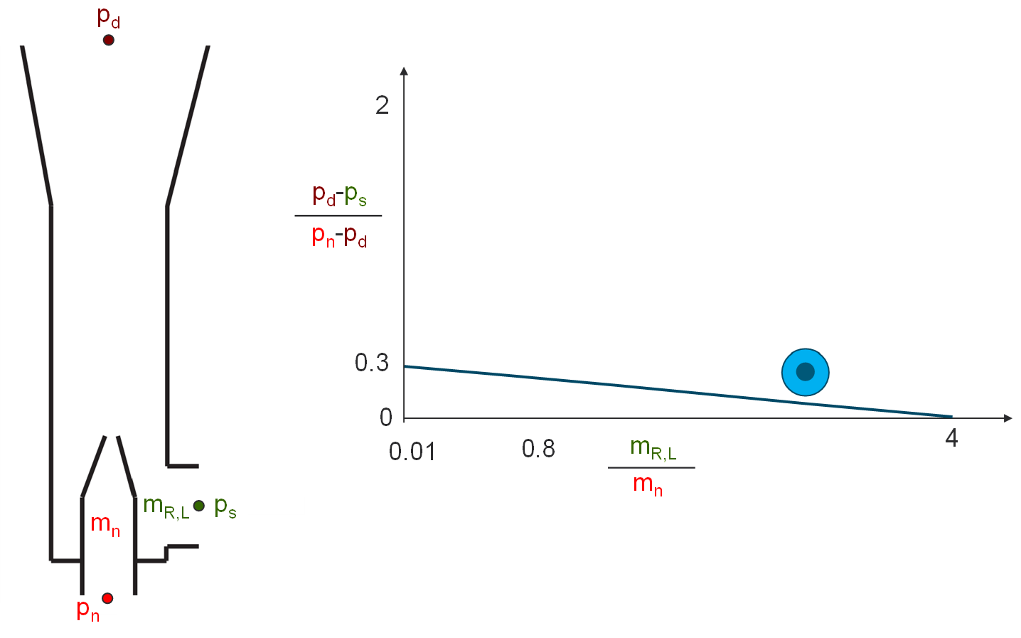
A jet pump exhibits a performance map like the one shown in the figures below (here is pressure, is discharge, is suction, is nozzle, is mass rate, is reservoir, and is liquid). whitson+ uses the performance map equations of SNAP, which depend on the nozzle-throat area ratio, and pump manufacturer, and have a correction factor for viscosity of power and suction fluid. A scaling factor can be used to alter the performance map if measured data is available.
A small annular section allows the pump to achieve high pressure differences but constrained to low flow rates, whereas a large annular section produces low pressure differences but constrained to high flow rates.
3.2.5.2. Calculation modes
Consider the well diagram shown in the figure below. In this configuration, power fluid is injected through the tubing, and reservoir fluids are brought to the surface through the annulus. In Whitson+, we first calculate the jet pump suction pressure and then determine the bottomhole pressure (in this case, using the flow path indicated by the number 1 in the figure).
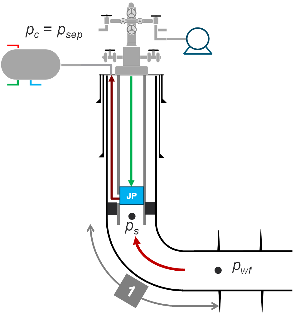
Whitson+ uses two methods to calculate jet pump suction pressure:
| Scenario | Description | Input Parameters Used |
|---|---|---|
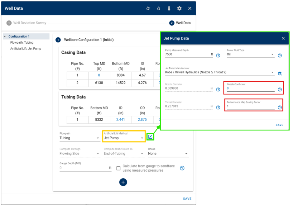
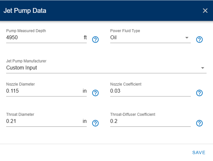
| Method 1. Power fluid surface pressure and rate provided | Only the nozzle equation is used (Bernoulli’s principle). If it returns a negative suction pressure, it defaults to Method 2. | Nozzle coefficient |
| Method 2. Only power fluid surface pressure provided | Power fluid rate and suction pressure are calculated using the performance map and auxiliary equations to ensure physical behavior*, following the method outlined in [6] with corrections for PVT fluid behavior. | Nozzle coefficient and performance map scaling factor |
-
As long as the calculation option is ON
-
No liquid cavitation and no gas choked flow in nozzle-throat annulus (equations described in [6])
If you have an accurate measurement of the power fluid rate, we recommend always entering it in the Production Data section so it can be used in BHP calculations. Note that Nodal and VLP calculations will always use Method 2.
About method 1
Small variations of power fluid surface pressure and rate can have a big effect on the calculated pump intake pressure and therefore on the calculated bottomhole pressure. The nozzle coefficient also has a big impact on the results.
About method 2
If you have low trust in your power fluid injection rates, you could remove those from the production data and let w+ calculate using power fluid surface pressure only.
Source of Power Fluid Surface Pressure Value
The value of power fluid surface pressure is taken from the column with the same name in production data. If missing, depending on the specified flow path, it will use tubing head pressure (flowpath: annulus, power fluid injected through tubing) or casing head pressure (flowpath: tubing, power fluid injected through annulus).
IPR-VLP intersection in Nodal not matching current operating point?
If you do BHP calculations using both power fluid surface pressure and rate and then run the nodal module, the IPR-VLP intersection will most likely not match the rate-bottomhole pressure combination calculated in the BHP module. This is because the BHP calculation was performed using only the nozzle equation, with given power fluid rate, while the VLP in the Nodal module is calculated with power fluid surface pressure and the jet pump performance map. The magnitude of the mismatch will depend on how closely SNAP's performance map matches the installed jet pump performance. A workaround is to adjust the performance map scaling coefficient until the IPR-VLP intersection is closer to the BHP values.
3.2.5.3. Adjustment of nozzle and/or performance map scaling factor
The default nozzle coefficient and performance map scaling factor may not accurately represent the performance maps of all jet pump types and sizes on the market. If manufacturer data is not available, consider the following approaches:
-
Power fluid rates and pressure are provided: If you have BHP gauge measurements with the pump installed, adjust the nozzle coefficient in the calculations to better match the measured values.
-
Only power fluid pressure is provided: If BHP gauge measurements are available, adjust both the nozzle coefficient and performance map scaling factor to improve agreement with the measurements.
Allowed values of the nozzle coefficient are in the range -0.38 to 1.12. If the calculated suction pressure is lower than expected, try using a smaller value; if the calculated suction pressure is higher than expected try using a bigger value.
Using jet pump manufacturer summary reports to find values of nozzle coefficient and performance map scaling factor
When you acquire a jet pump, the manufacturer usually runs some calculations to determine a suitable design and estimate operational conditions. You can use this information to adjust Whitson+ nozzle coefficient and performance map scaling factor to replicate the manufacturer values. Steps are:
- Input all data points provided by the manufacturer (wellhead pressure, oil, gas, water rates, power fluid surface pressure and rate) as well production data. Create two versions of the same data point: one including the power fluid rate, and another one ignoring it. We suggest you to put all data points that have power fluid rate first and those without after.
- Calculate bottomhole pressure.
- For the data points that have both power fluid rate and surface pressure: Adjust the nozzle coefficient until the calculated values are similar to the reported values.
- For the data points that have power fluid surface pressure only: Adjust the performance map scaling factor until the calculated values are similar to the reported values.
If the manufacturer report reports pump intake pressure only, not bottomhole pressure, you need to set your top perforation depth to the pump intake depth (and neglect everything below this point) before executing this procedure. After you are finished, remember to revert back and use the actual well top perforation.
3.2.5.4. Setting up a jet pump lifted well
Typical workflow to set up a BHP calculation for a jet pump lifted well:
1. In the menu “Production Data”, include values of power fluid surface pressure and rate in your production data (or, alternatively, power fluid surface pressure only):

2. In the "Bottomhole Pressure" menu, under the "Well Data" card, select "Jet Pump" as the artificial lift method. Then specify the production flow path as either "tubing" (power fluid is injected through the annulus) or "annulus" (power fluid is injected through the tubing).
3. Using the “edit” button next to “Jet Pump,” provide the details of the jet pump (if oil, produced dead oil will be injected, if water, produced water will be injected).
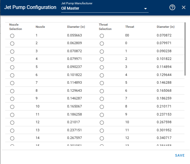
By clicking on “Jet Pump Manufacturer”, you can select from the following list:
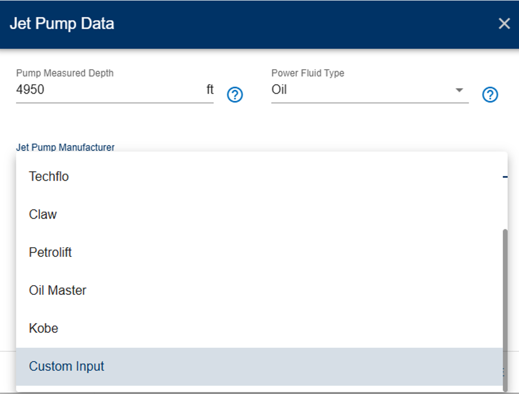
You will then be able to pick nozzle and throat sizes from the following options:
Behavior with gauge pressure
If gauge pressure is provided, the option to calculate from gauge is selected, and the gauge is below the pump, calculations will be performed from the gauge to the top perforation, ignoring the pump. However, if the jet pump is below the gauge, then the jet pump will still be used to calculate BHP.
3.2.5.5. Nodal analysis and jet pump
When running a nodal analysis with a jet pump, some VLPs might be incomplete (missing parts of the curve or missing entirely). This typically occurs because the pump cannot operate for some reservoir liquid rate values and is therefore not plotted.
3.2.6. ESP
There are two options to model ESP-lifted wells:
-
Calculation from pump intake sensor:
Set up procedure:
1. Your pump intake pressures are loaded into the Gauge Pressure (pwf, gauge) column,
2. Your wellbore configuration is loaded with the change in wellbore configuration from previous to ESP at the right 'Use From Date'.
3. Your wellbore configuration with ESP has a pump intake depth and 'Calculate from gauge to sandface using measured pressures' turned on. This computes the bottomhole pressure drop from the pump inlet to the top perforation - assuming the loaded gauge pressures record the pump intake pressures.
Finally, if everything, such as the pressure production data, looks okay and the pump is sized appropriately, the bottomhole pressure should show a smooth transition from previous wellbore configurations to flowing via ESP.
BHP Tuning Guidance
Be sure to not use these bottomhole pressures for tuning the correlations, this is why.
-
Calculation from wellhead using pump performance map: In this calculation mode, calculations are made from tubinghead pressure to pump discharge, then the pump performance map is used to compute pressure at pump intake, and then from pump intake to top perforation. Setup procedure:
1. In the "Bottomhole Pressure" menu, under the "Well Data" card, select "ESP" as the artificial lift method (the production flow path must be "tubing").
2. If a new window does not pop up immediately when selecting ESP, use the “edit” button next to “ESP” to provide the details of the ESP. It is possible to input several ESP models as part of the tubing string; use the button highlighted in purple below to add ESP models from top to bottom.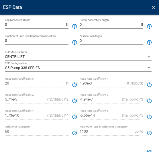
The area highlighted in red contains information common to all ESP models.
- Top measured depth is the measured depth of the pump discharge
- Fraction of free gas separated at suction, a number between 0 and 1. "0" means the full input surface gas rate is passed through the ESP. "1" means the ESP suction gas separator removes any free gas at the suction (corresponding to an amount "X" of surface gas rate separated). Any number F between 0 and 1 means that the pump will handle a standard gas rate of: input surface gas rate - F * X.
About input surface gas rate in BHP calculations
When there is a bottom production packer, all gas is forced to flow through the ESP; thus, the user should use a fraction of free gas separated at suction equal to 0. When gas is produced through the annulus, there are two options: 1. If the gas rate produced through the annulus and the gas rate produced through the tubing are measured, input only the gas rate produced through the tubing in the well production data, and use a fraction of free gas separated at suction equal to zero. 2. If only the total produced gas rate is measured (tubing + casing), input this value in the well production data and use a fraction of free gas separated at suction between 0 and 1. If measurements of pump suction pressure are available, vary the fraction until the match between calculation and measurement is acceptable.
The area highlighted in blue contains information specific to an ESP model.
- Pump assembly length, is the linear distance between ESP model discharge and pump suction.
- Number of stages, number of identical impeller-diffuser pairs in the pump assembly.
- Reference frequency.
- Head-rate coefficients: Pump performance of a single stage (head versus volumetric rate) is expressed as a 5th order polynomial. Operations at frequencies other than the reference frequency, are calculated by similarity laws. The user must either input manually the coefficients and reference frequency (by selecting "Custom Input" from the manufacturers list), or by selecting a manufacturer and pump model.
- Maximum rate at reference frequency: Every pump curve has a maximum rate allowed at reference frequency. This rate is either the inlet volumetric rate for which the value of head is zero, or a smaller value reported by the manufacturer.
Stage pressure boost is calculated sequentially, assuming isothermal conditions. When the stage is handling free gas, performance is calculated assuming a homogeneous mixture.
Manufacturer database
Selecting an ESP Manufacturer and ESP Configuration pulls the performance curves from the Manufacturer Configuration Database. If unavailable, choose Custom Input and enter the coefficients and reference frequency manually. To determine the coefficients you can paste 10 data points (rate-head pairs) into the following Excel file. Alternatively, you can send the ESP performance charts to support@whitson.com for us to add it to the database such that you don't have to add the information manually through the interface.
3.2.6.1. Recommended Practice for BHP Calculations for ESP-lifted wells
When estimating BHP, always aim to use the shortest and most reliable pressure path. If there is an ESP, but measured pump intake pressure is available and considered reliable, it is generally best to ignore the pump and calculate BHP directly from this pressure. Doing so minimizes assumptions, simplifies the pressure path, and improves accuracy.
Preferred Calculation Path:
- Pump intake pressure → bottomhole pressure
This direct approach is preferable to the more assumption-heavy path that includes an ESP:
- Wellhead pressure → tubing/casing pressure drop → ESP calculations → pump intake → bottomhole pressure
3.2.6.2. Nodal analysis and ESP
When running a nodal analysis with ESP, some VLPs might be incomplete (missing parts of the curve, especially towards high liquid rates). This typically occurs because it was found the pump cannot operate for some reservoir liquid rate values (they are above the maximum allowed) and it is therefore not plotted.
3.3. Dual-Conduit Flow
If the flow path is set to "Tubing and Annulus", the BHP is calculated by allowing the well stream to flow in through both annulus and tubing. The split of flow must be solved for by requiring that the pressure at the end of tubing is the same when calculating the pressure drop through both conduits, starting with casinghead pressure for the annular flow, and tubinghead pressure for the tubing flow.
3.4. Liquid Loading
3.4.1. Classical Critical-Rate Correlations
The Turner [1] and Coleman [2] critical rates are the classical correlations for predicting the minimum required gas rate to avoid liquid loading. These correlations can be used at all depths along the well. The correlations rely on a force balance on a liquid droplet to predict the minimum velocity needed to lift the droplet. The only difference between the two correlations is that Turner is 1.2 times Coleman.
The equation for the Coleman critical velocity is
where \(C\) is a unit conversion factor (1.5935... in field units), \(\sigma_{Lg}\) is the liquid-gas IFT, \(\rho_L\) is the liquid density and \(\rho_g\) is the gas density.
Converting the velocity to rate is done by where is gas holdup, is the hydraulic area, and is the gas formation volume factor.
3.4.2. Critical-Rate Correlations Accounting for Well Inclination
A modification to the Coleman critical velocity was made by Belfroid[3] to account for the well inclination. This is useful if the critical rate is computed at a different depth than the wellhead. The modified velocity is: where \(\theta\) is the inclination (deviation from vertical).
Application of Belfroid's Correction
The correction could be applied to both the Turner and Coleman critical velocities. In whitson+, Belfroid refers to the modified Coleman critical velocity/rate.
Nagoo[4] suggested a different correlation entirely where is a unit conversion factor (0.53244... in field units).
About Nagoo's critical gas velocity model
Nagoo has mentioned that, "...for horizontal gas wells use my equation in the casing below EOT, at about 80-85 degs", do not use at EOT.
Both these velocities are converted to rate using Eq. (\ref{eq:rate})
Which Critical-Rate Correlation to Use?
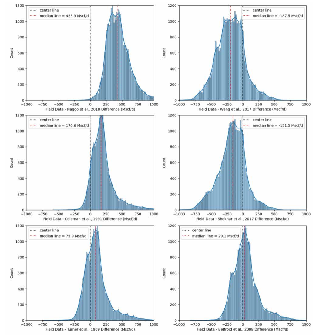
In 2022, Rahmati et al. [9] tested 6 critical rate correlations (Turner, Coleman, Belfroid, Wang, Nagoo, and Shekhar) on a dataset of 32,292 points of liquid loading onset, originating from 394 horizontal plunger-lifted gas wells in Canada and the United States. The tubing diameters were in the range 4.78 to 1.995 inches. Liquid loading was determined by plotting casing head pressure and gas rate during the plunger lift cycle and finding the corresponding gas rate when casing pressure reached a minimum (which also coincided with a significant decrease in the gas rate slope).
The figure below (taken from the paper) shows the histogram of differences between the critical rate correlations and the actual value. The spread was similar between the correlations. Wang and Shekhar were too pessimistic (predicted critical rates higher than actual), while Nagoo and Coleman were too optimistic (predicted critical rates lower than actual). Nagoo had a bias almost twice that of the other correlations. Belfroid and Turner are the most accurate, with Belfroid being slightly better.
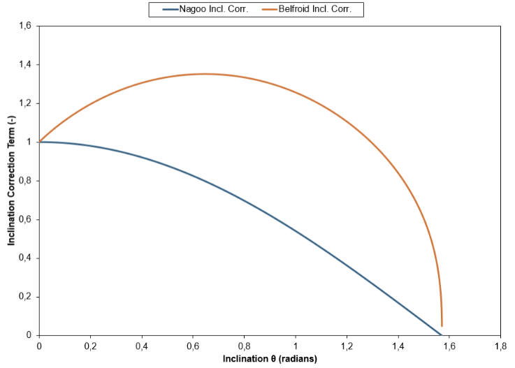
Nagoo's expression of critical velocity is derived following an approach very different from the one followed by Turner, Coleman and Belfroid. Contrary to the rest, Nagoo's expression is a function of inner pipe diameter, so smaller pipe diameters will give small critical rates. Moreover, the correction term from inclination is very different from Belfroid's (see the graph below, correction term versus pipe inclination angle from vertical).
3.4.3. Identifying Liquid Loading in whitson+ using Critical Rate Correlations
You can use the critical rate correlations above to see if the well is liquid loaded in the BHP feature itself.
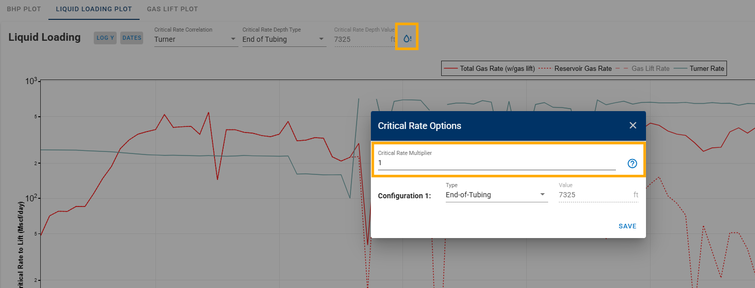
Click on the 'Liquid Loading' tab in the BHP feature and choose the following:
- Critical Rate Correlation: to calculate and plot the minimum gas rate required at the critical rate depth to avoid liquid loading. Choose between Turner, Coleman, Nagoo, and Belfroid - the plot should update with the chosen correlation. You can switch between these without having to recalculate BHP if these are already calculated once.
- Critical Rate Depth Type: Depth at which this correlation is used to calculate critical rate. Ensure that the BHP is calculated at least once and every time the critical rate depth is changed, to ensure the critical rate is recomputed for the right depth. Default critical rate depth, for consistency, is 'End of Tubing' for all wells. For wells without tubing in the wellbore configuration, the default critical rate depth will be 'Top Perforation' instead.
- Critical Rate Multiplier: Multiplier applied to all calculated critical rates for liquid loading. Use this to account for field-specific calibration. For example, enter 1.1 if actual critical rates in your field are consistently 10% higher than the Turner-calculated rates.
Why is the default critical rate depth 'End of Tubing'?
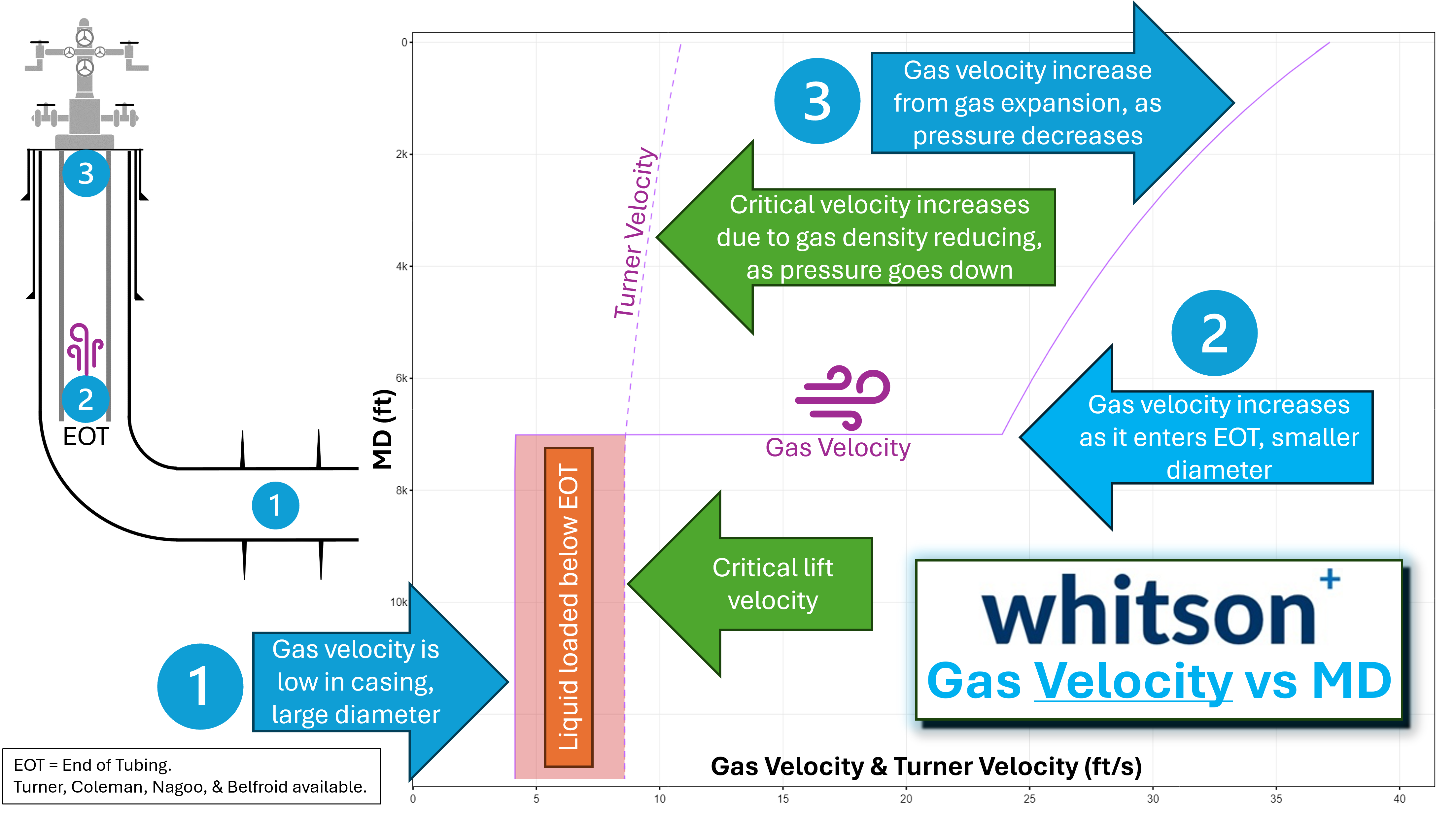
Within the tubing, the pressure is highest at the End of Tubing (EOT), and therefore the gas velocity is the lowest at the EOT. This is the location, within the tubing, we are most at risk for liquid loading. In short, if we are able to lift liquids at the EOT, we are guaranteed to lift liquids at every depth above the EOT in the tubing, due to the pressure decreasing and the gas velocity speeding up. Alternatively, we may be above the critical lift rate at the surface, but that tells us nothing about whether we're liquid loaded deeper in the wellbore.
BHP Calculation Dependency for Critical Rate Correlation
Ensure that the BHP is calculated at least once and an appropriate 'Bottomhole Pressure to be used in calculations' is also chosen because the critical rates will change accordingly. You need to strictly use one of the correlations for calculating critical rates so if you have 'Measured pwf, gauge' or 'Custom pwf' selected in 'Bottomhole Pressure to be used in calculations', they will default to Hagedorn and Brown.
Critical Rates can be calculated for the following critical rate depth types:
| Depth Type | Description |
|---|---|
| Wellhead | Critical rate is computed at the wellhead, i.e., at surface (depth of 0 ft). |
| Top Perforation | Default if tubing is absent – Critical rate is computed at the top perforation depth (as entered in the well data card). |
| End of Tubing | Default if tubing is present – Critical rate is computed at the end of tubing, i.e., at the tubing intake (as per the wellbore configuration). |
| Maximum Rate | Critical rate is calculated at all depths and the reported rates are the maximum rates calculated (at variable depths) throughout well history. |
| Specified | Using this option, you can manually specify the fixed depth at which critical rates are to be computed throughout well history. |
| Multiconfig | To compute the critical rate at different depths, specific to each wellbore configuration, across well history. |
Visualizing Pressures on the Liquid Loading Plot
You can toggle pressures on and off (using the 'Show pressures' button to the top-right of the liquid loading plot) to view the currently used bottomhole pressure, casing and tubing pressures and the difference between them on the same plot.
3.4.4. Critical rate correlations in nodal analysis
Here's an example well use case justifying the use of 'End of tubing' as the critical rate depth and quantifying the gas rates needed to prevent liquid loading using the Turner correlation:
In terms of critical velocities:
In terms of critical rates:
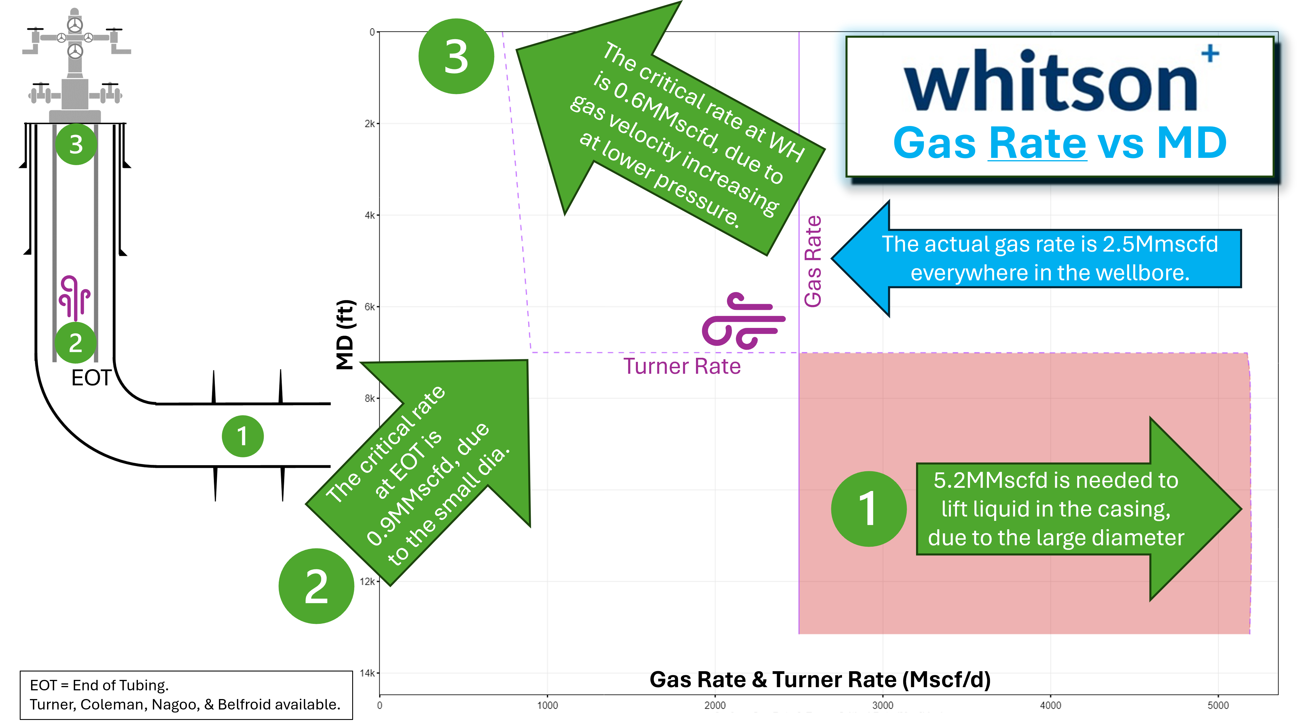
You can compute the critical and superficial velocity/rate vs depth and generate these plots in the Gradient tab of the Nodal Analysis feature for your wellbore.
3.4.5. Identifying Liquid Loading - Some practical tips
Two typical signatures of a well experiencing liquid loading are:
- The gas rate drops without a change in the wellhead (casinghead and/or tubinghead) pressures.
- The casing-tubing goes from flat to increasing (casing pressure minus tubing pressure is pretty flat when unloaded, once loaded, the tubing pressure starts to fall, so the delta between casing and tubing goes from flat to increasing).
3.4.6. Why is the critical gas lift rate under the gas lift optimization tab (Nodal) different than the critical rate shown in the BHP module for this day?
The workflow to calculate critical liquid loading rate is to first run a BHP calculation, with the given gas (and input lift gas rate, if any). Then, at the specified location (EOT, top perforation, etc.), one uses the method equation to estimate critical velocity (depending on whether using Turner, Coleman, Belfroid, or Nagoo). Lastly, one converts the velocity to rate by where is gas holdup, is the hydraulic area, and is the gas formation volume factor.
Since these equations use fluid properties like liquid and gas density, interfacial tension, and gas volume factor, they depend on the pressure and temperature at the location that is an output of the BHP calculation. The equation also uses the gas holdup (), which also depends on the output of the BHP calculation.
Consequently, the value of the critical liquid loading rate will change (sometimes significantly, sometimes slightly) as a function of the BHP calculation input. Even if one keeps almost everything constant (WHP, GOR, etc.) and just varies the rate, the output critical rate could still change.
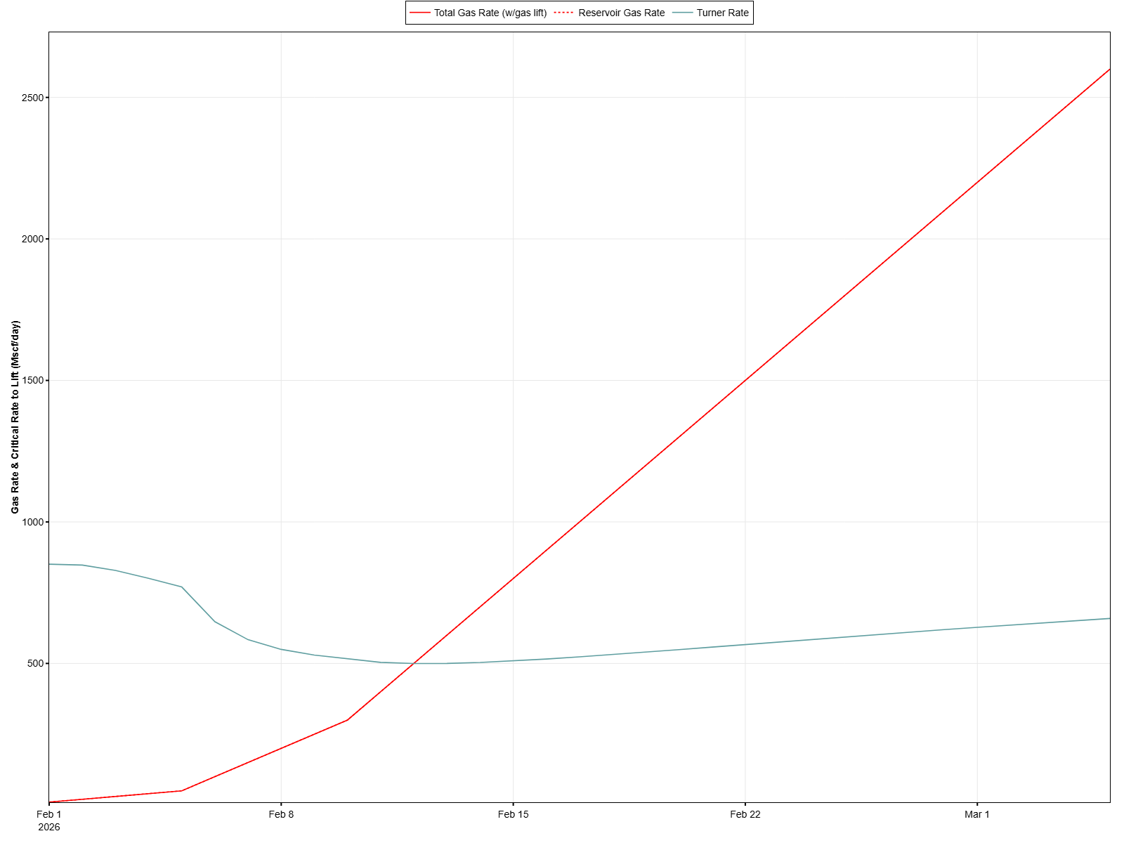
As an example observe the graph below showing the results for a synthetic case (vertical gas well, OGR = 200 stb/MMscf, 2.441 ID tubing @ 7000 ft, 4.778" ID casing @ 7100 ft (top perf), WHP = 100 psia, no water production ). There is no gas lift rate, only reservoir gas. Reservoir gas rates (red curve) are ramped up from 10 to 2600 Mscf/d, keeping all other variables constant. The dark blue-ish curve shows the values of critical rate at end of tubing calculated for each of the input gas rates. There is considerable variation in the critical gas rates calculated (from 850 to 500 Mscf/d). Dates where the red curve is below the blue, means the well is loaded, dates where the red curve is above the blue, means it is unloaded. From this plot, it seems that the critical reservoir gas rate to avoid loading is around 500 Mscf/d.
The results shown in the plot above were plotted in Excel to show calculated critical rate versus reservoir gas rate. Consider that you are currently producing 100 Mscf/d from this well (purple line in the plot below). The liquid calculation tells you that the critical gas rate is 650 Mscf/d. If you then increase the gas rate to 650 Mscf/d (green line on the plot below), you see that the critical rate is actually 500 MScf/d, NOT 650 Mscf/d. So you are overproducing to get rid of LL.
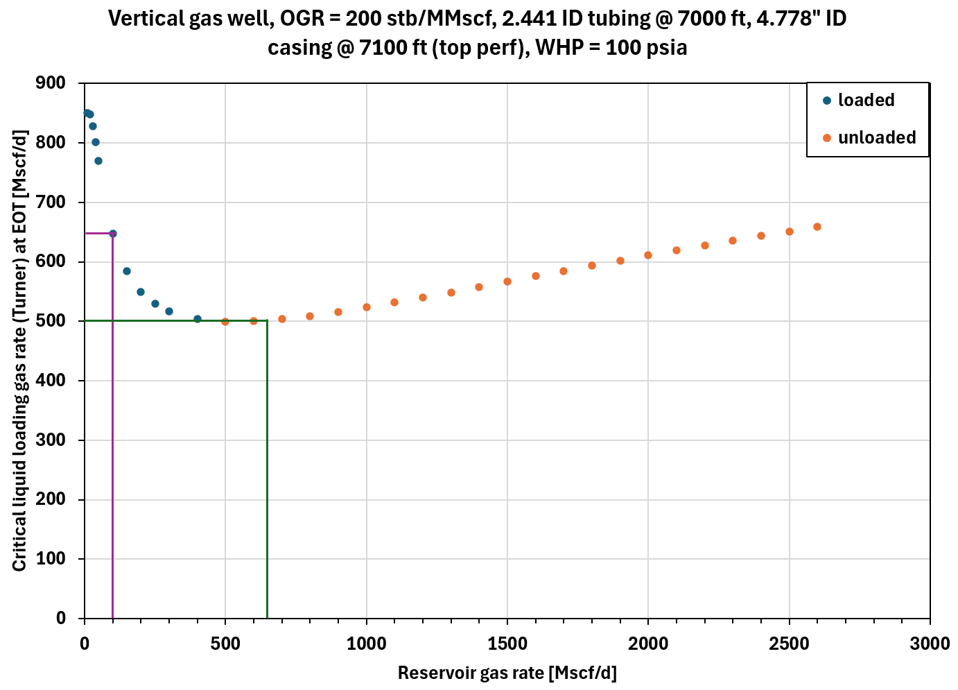
In some sense, the predicted critical rate is sort of a moving target, and it is only exact when you are on it.
In the gas lift optimization (GLO) module, since we are changing lift gas and reservoir gas rates, we calculate for each point in the gas lift performance curve the critical rate and we compare against the reservoir gas rate + the lift gas rate (depending on the LL location the user specifies specified). The curve is then made discontinuous or continuous depending on the result of the comparison. This is similar to what was done in the figure above.
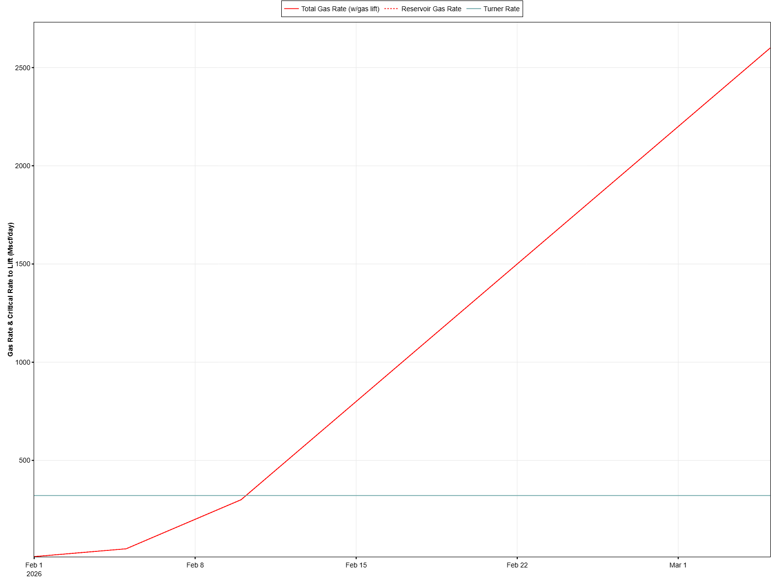
The plot below shows the result of the GLO module for this well for the first date (gas rate = 10 Mscf/d). You see that the gas lift injection rate where it stops being loaded is around 380 Mscf/d (total rate 380 Mscf/d + 13 Mscf/d reservoir rate ~= 400 Mscf/d).

Why does this number not match the 500 Mscf/d value discussed earlier? This is because when one injects lift gas, the gas oil (gas-liquid) ratio of the fluid in the tubing is increasing as a function of the amount of lift gas and above reservoir GOR. Since the GOR is higher this affects the flowing pressures in the tubing, liquid holdup, and related properties, ultimately affecting the value of the critical liquid loading rate.
Variation of liquid loading critical rate when location is wellhead
When the liquid loading location is wellhead, usually pressure and temperature are constant, so most inputs to the critical rate calculation (densities, interfacial tensions, gas volume factor) will be constant. However, the calculated critical rate could still vary if there are variations in gas liquid ratio (GLR). GLR changes cause changes in liquid holdup, which affects the conversion from critical velocity to critical rate. Consider the previous example discussed, but now the location of the critical velocity is set to wellhead instead of end of tubing. GOR and GLR are constant.
Summary: Often, the reported (calculated) value of gas critical rate is only exact when one is very close to loading conditions. If one is above or below, the value is approximate. But it can still be used as an indication of how much to increase (or decrease) the gas rates.
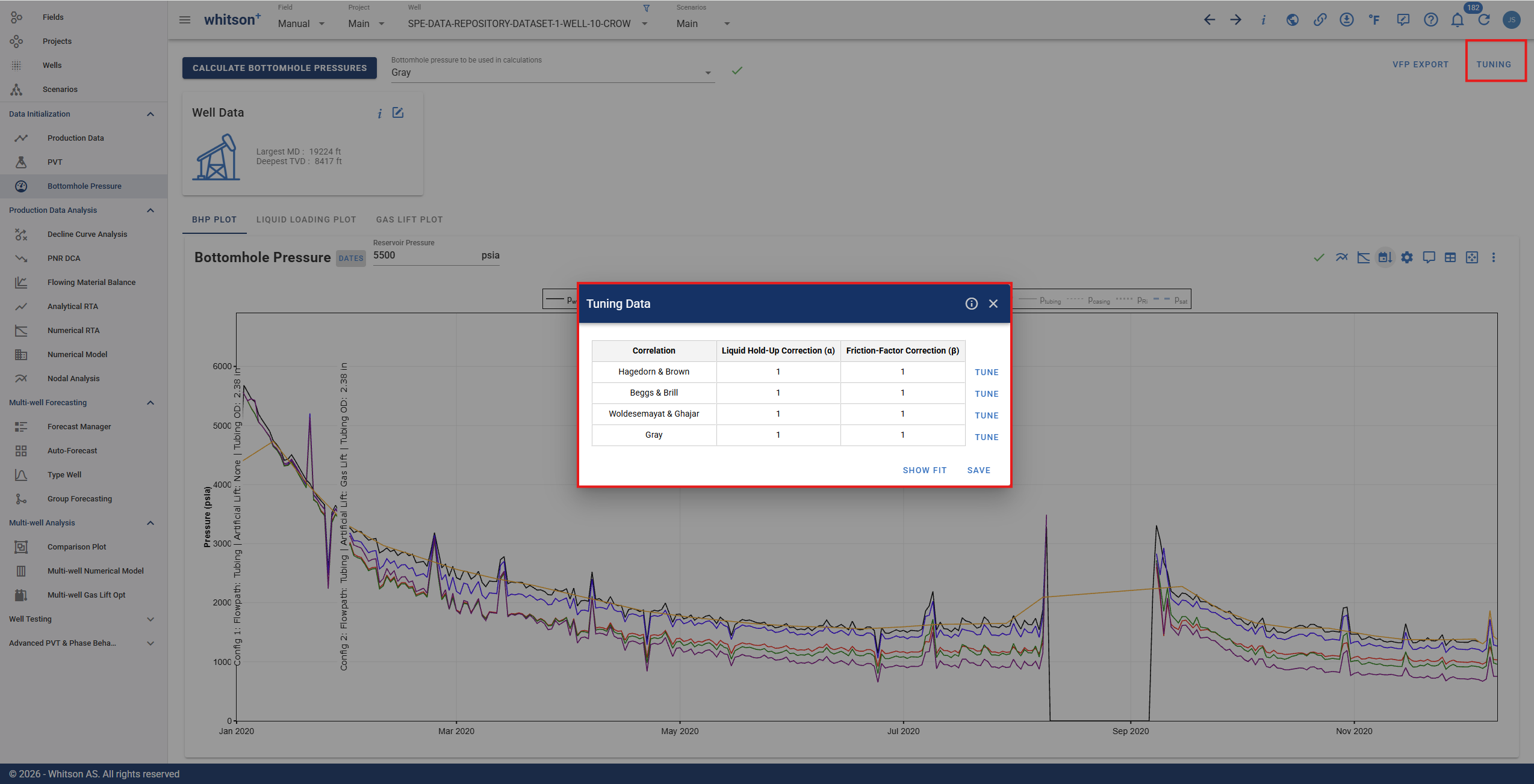
3.5. Correlation Tuning
The BHP tuning functionality can be accessed by clicking Tuning to the upper right of the BHP feature as seen below.
The following video illustrates a practical example of "BHP correlation tuning to measure gauge data"
3.5.1. Correcting the Properties
The multiphase-flow correlations used to compute the bottomhole pressure can be tuned in whitson+. This is achieved by correcting the liquid hold-up by a parameter \(\alpha\), and the friction factor by a parameter \(\beta\). Correcting the liquid hold-up affects mainly the gravity pressure drop, while correcting the friction factor affects the friction pressure drop. The corrections are made as follows:
Liquid Hold-Up Correction:
The liquid hold-up, \(H_L\), is always lower bounded by the liquid flux fraction, \(C_L\), and upper bounded by 1. To honor this bracketing in a tuning process, it is easier to convert the liquid hold-up into an equivalent slip velocity that is only lower bounded by 0, and then apply the \(\alpha\) parameter as a correction multiplier. The slip velocity is defined as
where \(v_g\) and \(v_L\) are the gas and liquid velocities, and \(v_{sg}\) and \(v_{sL}\) are the superficial gas and liquid velocities. Solving (\ref{eq:slipVelocity}) for \(H_L\), we get:
The liquid hold-up correction is made by
- Compute the slip velocity \(v_s\) from \(H_L\) predicted by the default/untuned correlation using Eq. (\ref{eq:slipVelocity})
- Multiply the slip velocity by \(\alpha\) to get \(v_{s}^{corr}=v_s\alpha\)
- Calculate \(H_L^{corr}\) with the corrected slip velocity \(v_s^{corr}\) using Eq. (\ref{eq:liquidHoldUp})
Friction-Factor Correction:
The friction factor is corrected by multiplying the calculated friction factor from the default/untuned correlation by \(\beta\).
3.5.2. Selecting the Measured Pressure Points to Tune
The tuning procedure includes a routine that selects a subset of the measured gauge data over time. This is done for two reasons, (1) to speed up the tuning process by computing less pressures points, and (2) to minimize the effect of outliers. The sampling procedure involves three steps:
- Remove outliers that have more than a 20% relative difference from their neighbors.
- Compute a moving average of the filtered data.
- Sample the moving average at a constant spacing of 20 days.
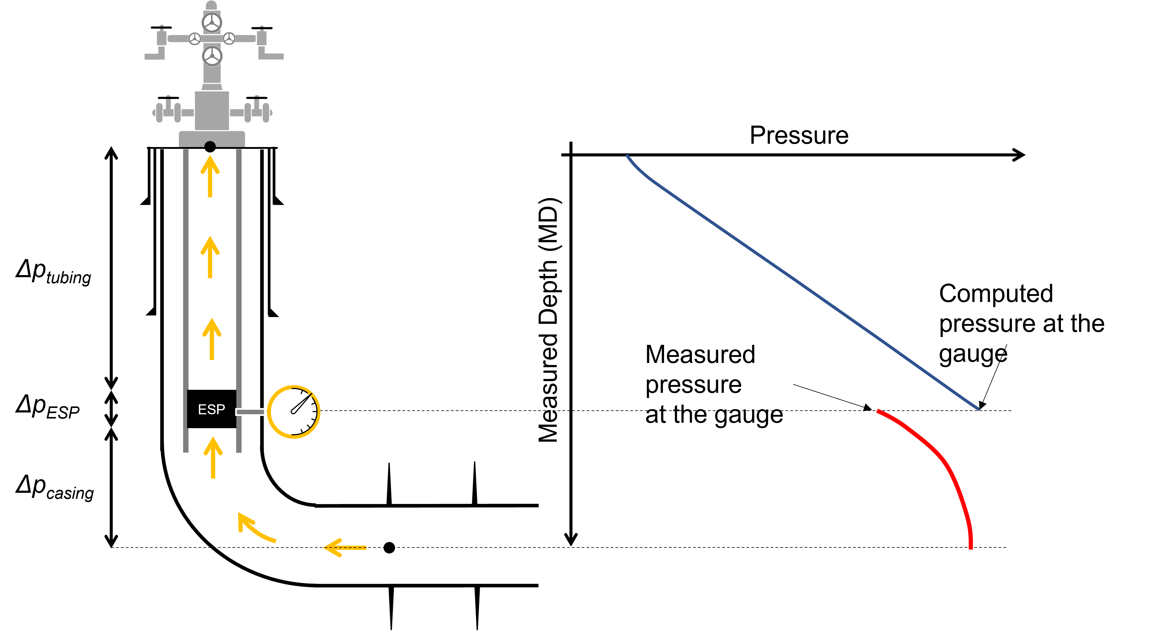
3.5.3. Correlation Tuning Using Measured Pressures from an ESP when using the calculation option "from gauge"
When using the ESP calculation option "from gauge", measured pressures at the suction of an electric submersible pump (ESP) should not be used to tune the bottomhole-pressure correlations. The reason for this is that the computed pressures from wellhead to gauge (situated at the ESP inlet) does not account for the delta-pressure caused by the ESP.
3.6. Estimating Initial Reservoir Pressure in whitson+
Here we are estimating reservoir pressure from flowing pressure and rate data, typically acquired for most wells. These are just approximation methods involving uncertainty and other tests, specific to this purpose, like Diagnostic Fracture Injection Tests (DFIT), downhole formation testing tools, pre-frac step-rate injection tests, post-frac instantaneous shut-in pressure combined with frac gradient relationships, opening pressure of the first port for packer/sleeve completions, etc., should be used wherever available.
In whitson+, the already available rates and pressure data can be used in two ways to estimate reservoir pressure:
3.6.1. Reservoir Pressure from flattening of flowback BHP before hydrocarbon production
This technique is outlined in Jones et al[5], (URTeC: 1934785), and consists of three steps to diagnose reservoir pressure from flowback data (preferably hourly):
- Calculate BHP for the flowback data using a suitable multiphase flow correlation.
- Plot BHP along with rate and other pressure data.
- Look for a flattening or minimum BHP, just before the first measurable hydrocarbon production is reported. Casing pressure might show a similar pattern too. This flat portion or minimum in the BHP curve is the estimated reservoir pressure.
Assumptions
Produced fluids during flowback are initially 100% water, with delayed hydrocarbon breakthrough. Flowback begins shortly after the frac job was completed and the frac plugs are drilled out.
This is so that there is the least uncertainty in the calculated BHP initially and the BHP at the beginning of flowback is higher than the estimated reservoir pressure, so the "frac charge" is not allowed to dissipate through leakoff (such as during an extended shut-in or installation of artificial lift after the frac job). Hourly flowback data makes it easy to identify the pressure behavior associated with first hydrocarbon production.
The simplest explanation for this might be that trace amounts of immeasurable hydrocarbons (due to relatively high water rate) start entering the wellbore and arrest the decline in wellhead pressure; hence, BHP tends to remain flat just before measurable hydrocarbon is separated from the flowback frac water and rates are reported.
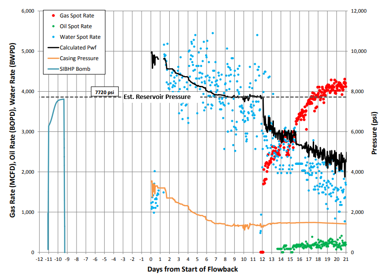
Example flowback data for estimation of reservoir pressure (from Jones et al., URTeC 1934785)
The flattening of BHP, identified as reservoir pressure, may be too short or completely missing if the drawdown is too aggressive, productivity is too low, finite conductivity fractures are present, near-wellbore skin damage is present, or large changes in choke occur instead of gradually and monotonically opening them. In these cases, the data has step changes in rates and pressures, or BHP drops quickly and significantly below the actual reservoir pressure - making it really difficult to identify reservoir pressure.
Visualizing BHP, Rates, and Surface Pressures
In the BHP feature, you can plot rates and pressures simultaneously, as outlined above by clicking the 'Show rates, surface pressures' button on the top right of the BHP plot.
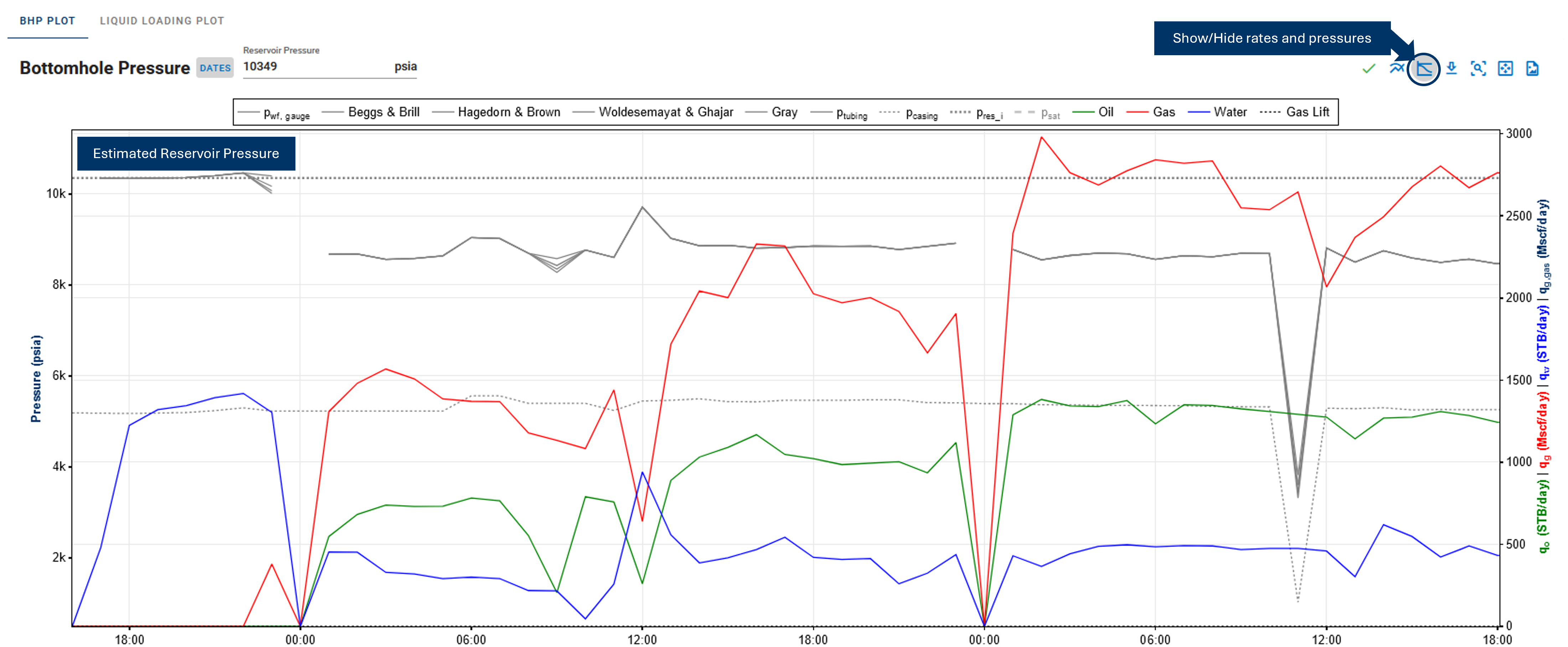
Be sure to zoom into the very early time section of the data and appropriately adjust pressure and rate axis limits on the plot to display a diagnostic plot similar to the one referenced from the paper.
3.6.2. Reservoir pressure from IPR
Here are the steps to estimate reservoir pressure from an approximate IPR fit to BHP vs. rate data:
- Calculate BHP for the pressure and rate data available.
- On the Bottomhole Pressure plot, click the 'Estimate Initial Reservoir Pressure' button in the top right. This opens a new dialog box allowing you to view BHP vs. rate plots, choose the IPR type and BHP correlation to use, and select the number of days of data to display on this plot.
- By default, oil wells will plot the calculated BHP vs. measured oil rate data for the first 10 days after oil breakthrough and use Vogel's IPR curve. For gas wells, the plot defaults to BHP vs. gas rate and uses C&n or the backpressure equation as the IPR type.
- Select at least two points with the lasso tool. The slope or productivity index and the saturation pressure (from the well's PVT) are used to set up an approximate IPR fit to the data.
- Extrapolation of this IPR to the y-axis (or the intercept) gives the initial reservoir pressure.
- Click Save to update the initial reservoir pressure for the well with this value.
These steps are shown in the GIF below:
3.7. Activate BHP Injection Mode
If you want to model the bottomhole pressure during an injection process, that can be done by activating the BHP injection mode. This is done in the Calculation Settings in the Well Data card as seen above. When enabled, this switch allows users to simulate the pressure at the bottom of the wellbore during injection. All uploaded rates (e.g. oil, water, or gas) will be assumed to be injected rates.
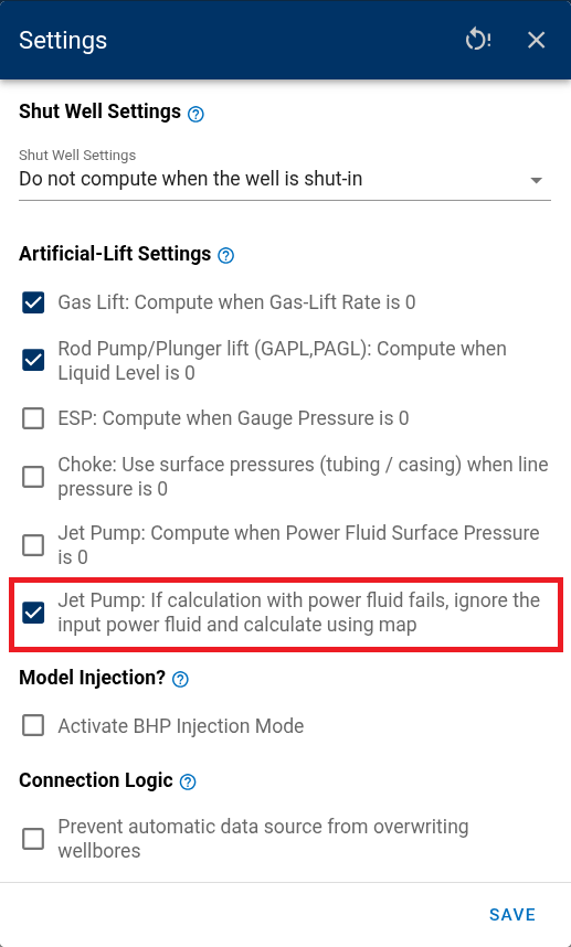
3.8. Shut-in Well Settings
Select whether the BHP calculator should skip or compute the BHP on days when the well is shut (i.e., all rates in the production data are missing or zero).
The shut-well BHP can be calculated by assuming a gas-filled well or by using a specified gradient.
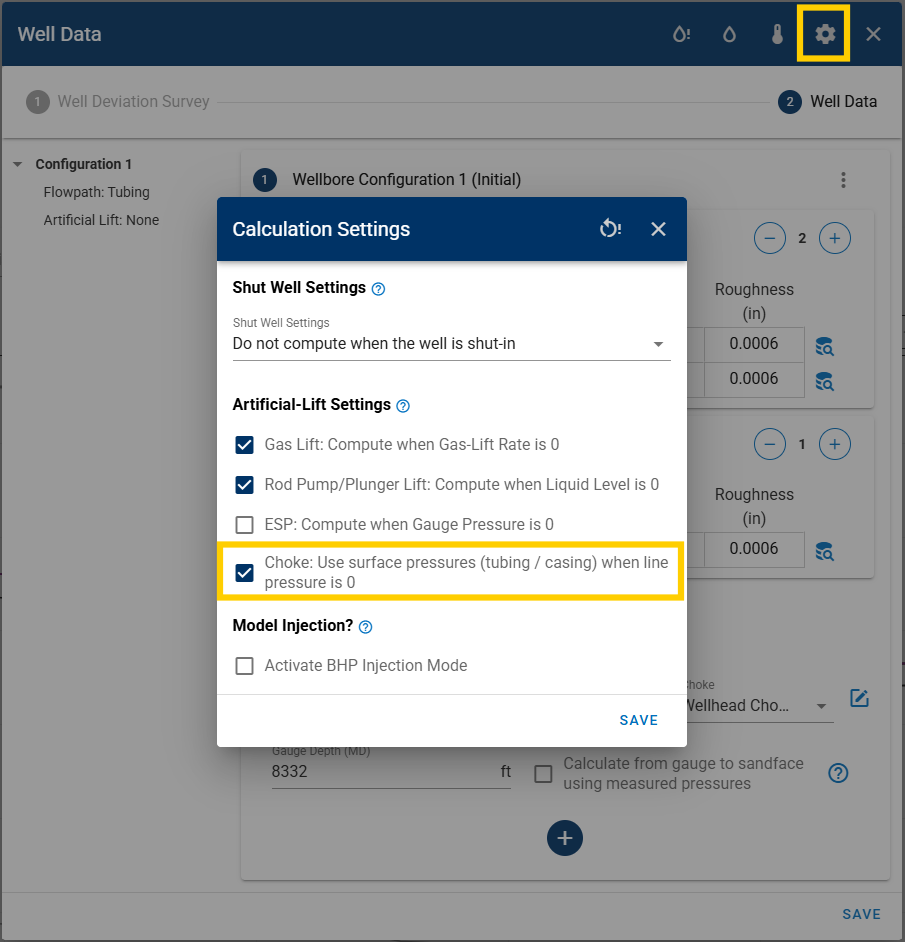
3.9. Choke
The choke setting represents a pressure restriction point in the wellbore or surface facility and determines the pressure drop between two points in the system. This is typically between the wellhead and surface flowline, or at a specified downhole depth. Each wellbore configuration includes one choke settings such as choke coefficient, choke depth, and choke size.
What is Choke Coefficient?
The Choke Coefficient is a correction factor used to account for vena contracta effects and irreversible energy losses. This coefficient can be estimated using single-phase valve coefficients provided in manufacturer datasheets, or more accurately determined through field calibration with measured field data.
When configuring a choke in whitson+, it is important to understand which pressure reference is required depending on where the choke is located:
-
For wellhead chokes, the line pressure should be used. Otherwise, you can choose to fall back on tubing or casing pressure using the toggle shown below. Moreover, note that the choke depth is always zero and the choke size is fetched from production data.
-
For Downhole Choke, the default tubing or casing pressure is used. The choke depth and size (opening) are required. If choke size changes with time, user can add new configurations and edit the size for those configurations.
Operational Envelope
A fixed opening wellhead or bottom-hole choke will display the performance curve (pressure drop vs. surface oil or gas rate), shown in the figure below.
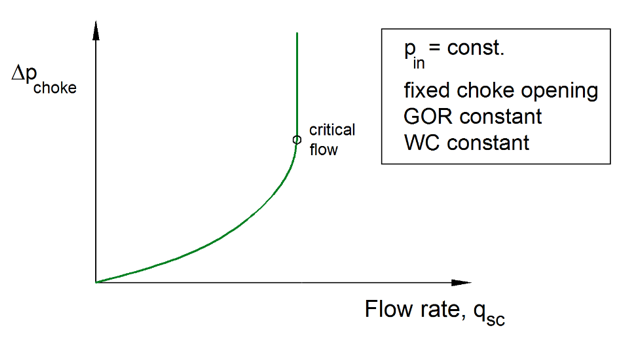
This curve is generated by keeping the inlet pressure, GOR, and WC constant, while changing the downstream pressure from the inlet pressure value to atmospheric conditions (see the sequence plotted in the animation below).
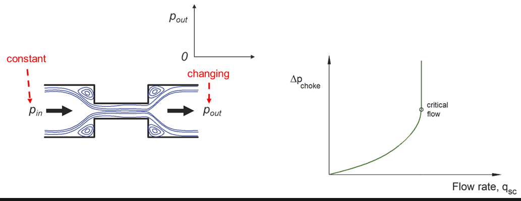
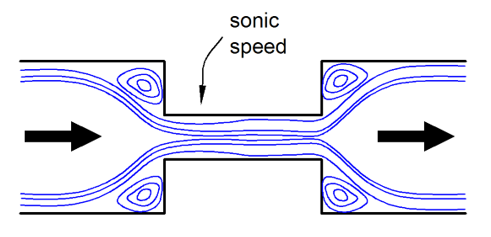
The pressure drop across the choke increases in a non – linear manner when the rate is increased. However, there is a point where it is not possible to increase the rate further (i.e., the pressure downstream the choke does not impact the rate flowing through the choke). This is because the fluid velocity at the throat of the choke has reached the sonic velocity. This typically occurs when the pressure ratio is between 0.5-0.6.
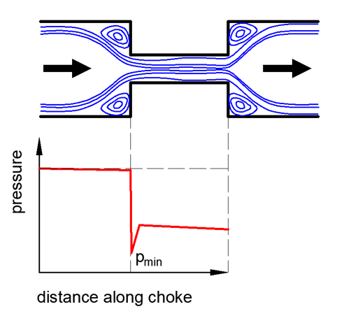
The figure below shows the behavior of pressure along the axis of a bean choke. Note that pressure drops suddenly when the flow encounters the contraction point. In gas-dominated flows this sudden pressure reduction can cause cooling (due to the Joule-Thomson effect), liquid condensation and ice formation (in the presence of free water).
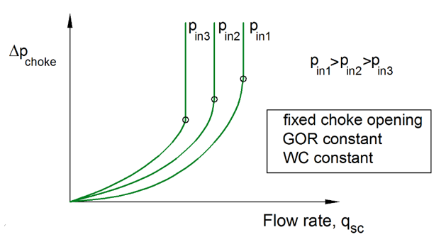
The figure below shows the performance curve of the choke when the inlet pressure is varied. The pressure drop at which the critical flow is reached increases proportionally with the inlet pressure: . Changes in GOR and WC give a similar variation of the performance curve.
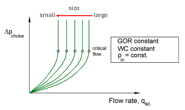
The figure below shows the choke performance curve for 5 different choke openings. A smaller opening will provide a larger pressure drop than a larger opening, and critical flow will be reached at lower flow rates.
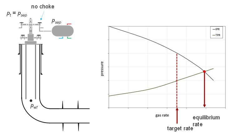
Choke Planning Using Nodal Analysis
Consider the situation shown in the figure below. A nodal analysis is performed at the bottomhole on a well with no wellhead choke. The equilibrium rate is higher than the target rate; therefore, choking is required.
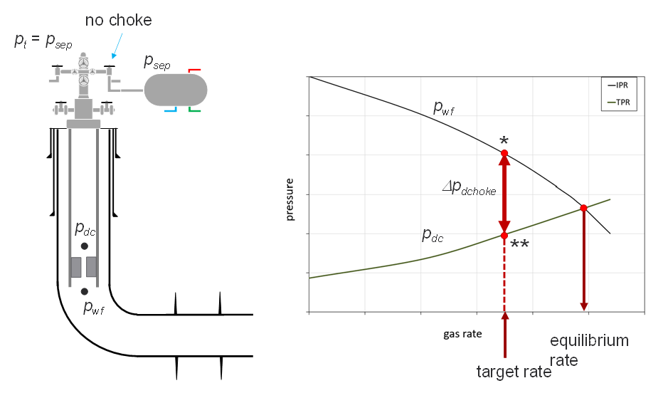
If a bottom-hole choke is used, the choke must drop the pressure from the pressure available from the reservoir (marked with * in the figure) to the pressure required to flow to the surface through the tubing (marked with ** in the figure).
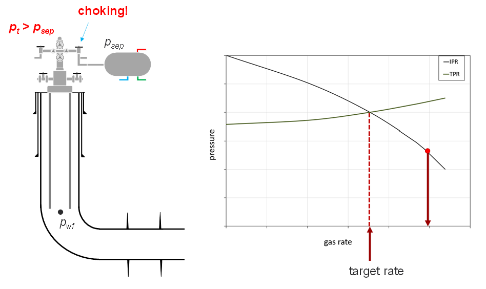
Another alternative is to use wellhead choking (shown in the figure below). In this approach, wellhead choking increases the tubing head pressure and “shifts” the TPR up, moving the intersection to the left.
Choke Modeling
Chokes are often modeled by integrating the differential version of the momentum equation between the choke inlet and the throat and assuming no friction or localized losses between these two points. Due to the convergence of the flow, the effective throat cross-section area (often referred to as vena contracta) is not exactly equal to the throat cross-section area (), thus a correction factor () is introduced () and is often varied in the range (0,1] such that the model predicts accurately measured data.
The one-dimensional momentum equation in differential form for liquid-gas flow, neglecting friction and localized losses, is:
where is holdup, is velocity, is density, and pressure.
The whitson+ model assumes liquid and gas travel at the same velocity (mixture velocity, , equal to the sum of local rates of oil, gas and water divided by cross-section area). Then, the equation above is integrated between the inlet and the throat, while neglecting inlet velocity, to obtain:
is the homogeneous mixture density, defined as:
where is the gas mass fraction, and , are the gas and liquid phase densities, respectively.
Calculation Details
In all whitson+ applications like bhp calculations and nodal analysis, rate across and pressure downstream the choke are known, and it is desirable to find inlet pressure.
The equation is solved by computing numerically the homogeneous density integral, assuming isothermal flow and thermodynamic equilibrium. However, there is some care to be exercised about the pressure value to employ at the throat.
When operating in the subcritical regime, the pressure downstream of the choke is usually employed to approximate the pressure at the throat, assuming there is very little pressure recovery after the throat. When operating in the critical regime, the pressure measured downstream of the choke is lower than the pressure at the throat and is initially unknown. The main challenge is that often it is not known beforehand if the choke is operating in the critical or subcritical regime, so the calculation requires some trial and error.
As an example, consider the flow of dry gas through a choke, outlet pressure equal to 50 bara, inlet temperature 80 °C. The figure below shows the value of the residual of the choke model for a rate of 1e6 Sm3/d, and for several combinations of inlet pressure and throat pressure values, from 50 bara to 500 bara. Cases where the inlet pressure is lower than the throat pressure are discarded. The black line is the inlet-throat pressure combinations where the residual is zero (potential solutions to the choke model). The physical solution is the minimum point in the black curve. When the minimum lies when the throat pressure is equal to the downstream pressure, the choke operates in the subcritical regime. Otherwise, the choke operates in the critical regime (like in the figure below).
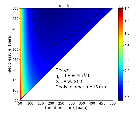
Recommended Practice for BHP Calculations
When estimating BHP, always aim to use the shortest and most reliable pressure path. If there is a wellhead choke, but measured tubing head pressure or casing head pressure is available and considered reliable, it is generally best to ignore the wellhead choke and calculate BHP directly from this surface pressure. Doing so minimizes assumptions, simplifies the pressure path, and improves accuracy.
Preferred Calculation Path:
- Tubing/casing head pressure → tubing/casing pressure drop → bottomhole pressure
This direct approach is preferable to the more assumption-heavy path that includes a wellhead choke:
- Line pressure → wellhead choke pressure drop → tubing/casing head pressure → tubing/casing pressure drop → bottomhole pressure
This distinction is especially important when high-confidence surface pressure data is available — performing wellhead choke calculations in such cases may unnecessarily introduce uncertainty.
When Downhole Gauge Data Available
If a downhole pressure gauge is available, it is best to use that data directly for BHP estimation. This eliminates the need for pressure gradient assumptions and calculations entirely, resulting in the shortest and more reliable output.
When to Use Wellhead Choke-Based Calculations
- Surface pressure is unavailable or unreliable, but line pressure and flow rates are available.
- Line pressure and surface pressure are available, but flow rates are unavailable or unreliable (an iterative approach will be used to adjust rates until the calculated surface pressure matches the measured value)
- Simulating or designing choke strategies for operational optimization, such as evaluating pressure response or production control, erosion mitigation, etc.
Estimating Choke Size from Cv
When working with adjustable chokes, manufacturers often provide a value of flow coefficient Cv for different openings (position, usually in %). whitson+ requires choke size in 1/64 in as input. You can use the following equation to convert from Cv to choke size in 1/64 in:
Manual Calibration of Choke Coefficient (wellhead choke)
If you have values of wellhead pressure, line pressure and rate, you can use them to tune your choke coefficient, such that the accuracy of your choke calculations is improved. To do this, go to the feature "gradient" in the "Nodal Analysis" module. Select the date you want to do the calibration for. Wellhead pressure (either tubing or casing head pressure, depending on the flow path) is an output of the calculation. Adjust the choke coefficient manually until the wellhead pressure output of gradient calculation matches the measured value of wellhead pressure.
Manual Calibration of Choke Coefficient (bottomhole choke)
If you have a bottomhole gauge, you can use it to tune your choke coefficient, such that the accuracy of your choke calculations is improved. To do this, go to the feature "gradient" in the "Nodal Analysis" module. Select the date you want to do the calibration for. The calculation outputs pressure versus depth, and one can read pressure at gauge depth. Adjust the choke coefficient manually until the gauge pressure output of gradient calculation matches the measured gauge value
3.10. Vertical Flow Performance (VFP) Export
VFP tables are used to model the well's VFP under a range of flowing conditions, without requiring BHP to be recalculated for every individual parameter set. Instead, simulators can interpolate the parameters based on defined combinations of key input variables.
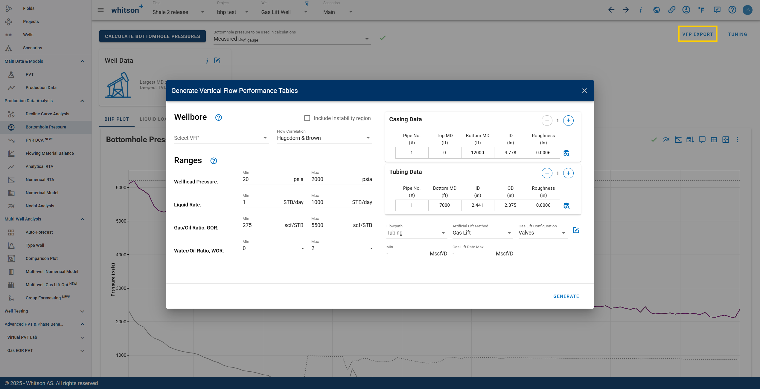
The VFP Export feature in whitson+ generates a sensitivity-based table in ECLIPSE-compatible format, allowing users to import it directly into their software.
To generate the VFP sensitivity table, the user must specify:
-
Well configuration (tubing, deviation, depth, etc.).
-
Surface pressure, liquid rate, GOR and WOR limits.
-
BHP Flow Correlation.
File Output
Once the necessary inputs are provided, the export will generate a file with structured combinations of the input parameters. A preview of the output format is shown below:
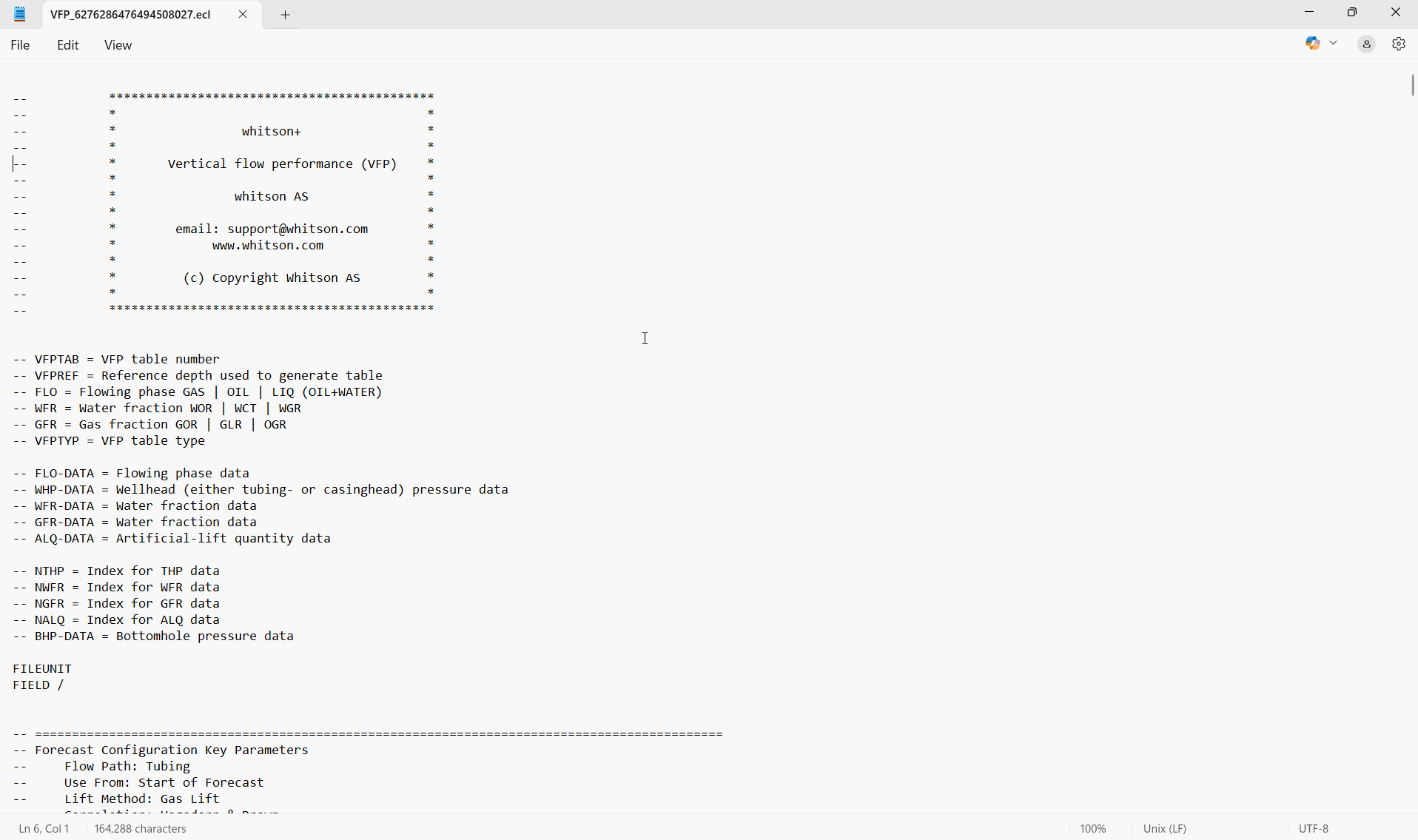
By default, the generated table includes:
- 25 points for flow rates
- 10 points for wellhead pressure
- 5 points for WOR/WGR
- 8 points for GOR/CGR
- 3 points for gas lift injection rate (if applicable).
All points are linearly spaced within the defined minimum and maximum range. The final VFP table includes all valid combinations (sensitivity mix) across the defined ranges.
VFP Export Output
- The VFP table format is compatible with ECLIPSE simulators only.
- Each table is well-specific and sensitive to the wellbore design, trajectory, artificial lift, and fluid properties.
3.11. Erosional velocity
whitson+ has the capability to estimate maximum erosional gas rates in wells at key or user-specified locations, following a similar logic to the liquid loading critical velocity calculations. There are two methods available:
3.11.1. API RP 14 E
The API recommended practice (RP) 14 E [7] is the classical and most popular method to predict the maximum allowable fluid velocity to avoid erosion in conduits carrying two-phase gas liquid flow. The origin of the equation is debated, ranging from theoretical to purely empirical, and there have been several studies reporting on its limitations. Most of the criticism is because erosion is a complex phenomenon that depends on several factors, and the API RP 14 E equation is too simple to account for all.
The equation is:
where is erosional velocity (ft/s), is the empirical constant (lb/(s ft), and is gas-liquid mixture density (in whitson+ the homogeneous mixture density is used, lb/ft³) at pressure and temperature.
The RP suggests, for solids-free fluids, using for continuous service and for intermittent service. It is reported that values up to 250 (intermittent) and 200 (continuous) have been used for solid-free fluids when using corrosion inhibitors or corrosion-resistant alloys.
In the presence of solids, is usually below 100. No guidelines on values are provided in the RP. The RP states that values must be defined and verified by periodic surveys.
3.11.2. Svedeman and Arnold
Since API RP 14 E does not provide recommendations of c values for flow with solids, a model that considers solid content (Svedeman and Arnold [8]) was implemented following recommendations from clients.
The equation is as follows:
where is erosional velocity (ft/s), is the pipe inside diameter, in, is the solids flow rate in ft/d, and is a fitting erosion constant. The equation is derived based on an allowable metal erosion rate of 5 mpy (thousands of an inch per year). A value of equal to 13 has been suggested by clients for tubing fluid/sand flow.
Note the erosional velocity is a function of sand rate and conduit inner diameter. Since the sand rate is constant along the conduit, it will change only if there is a change in cross section.
Use this model with care
A big source of uncertainty in this model is the value. Consider verification with surveys or studies.
Use this model with care
Erosional velocities predicted with this equation are usually quite low, and it is often the case that fluid velocities are above it. But what matters in erosion is the cumulative effect over time. For example, if there are only few days within the year with high sand production (and fluid velocities higher than the erosional limit) but it later drops to an acceptable threshold, the total erosion rate might still be way below the allowable 5 mpy.
3.11.2.1. Nodal analysis and erosional velocity calculations using Svedeman and Arnold
When conducting nodal analysis, while calculating the TPR curve and erosional velocity with the Svedeman model, it is necessary to calculate sand rates at varying oil (or gas) rates. The approach used in whitson+ is to first calculate the sand-fluid ratio
using values from the production data point. At other oil-gas surface rates it calculates the sand rate assuming the ratio remains constant (sand rate is proportional to reservoir fluids surface rates).
3.11.3. Conversion from erosional velocities to gas rates
Erosional velocities are converted to gas rates by the following equation:
where is gas holdup, is cross-sectional area, and is gas volume factor.
3.11.4. Identifying erosion risk in whitson+ using erosional rate correlations
You can use the erosional rate correlations above to see if the well has a risk of erosion in the BHP feature itself.
Click on the 'Liquid Loading Plot' tab in the BHP feature and choose the following:
- Erosional Rate Type: to calculate and plot the maximum gas rate allowed to avoid erosion. Choose between API 14E and Svedeman and Arnold - the plot should update with the chosen correlation (to get values with the Svedeman & Arnold model, remember you need to input sand rates in the production data). You can switch between these, without having to recalculate BHP if these are already calculated once.
To the right of the Erosional Rate Type: selector, there is an edit button, where the user can edit the following under the "Erosional" tab:
- Erosional model constants: Constants used in the erosional rate calculations. You can input different values and see the effect on the rate, without having to recalculate BHP if these are already calculated once.
- Location. For each well configuration the user has the option to select a preferred location where the erosional rate is calculated. If the user changes values here, a new BHP calculation is often required to update the values.
- Use custom diameter, outlets or scaling. Here the user can input a different diameter, number of channels greater than one, or a custom scale factor for each location. This is useful, for example, when wellhead flow is passing through two wing valves, and the internal diameter of the valves is slightly smaller than the tubing ID. You can input different values and see the effect on the rate, without having to recalculate BHP.
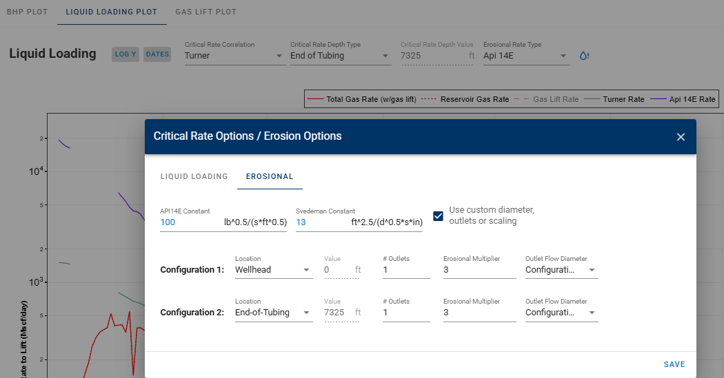
The image below shows how the correction to the 14E erosional rate is performed for different constants, diameters, numbers of outlets, or scaling factors.
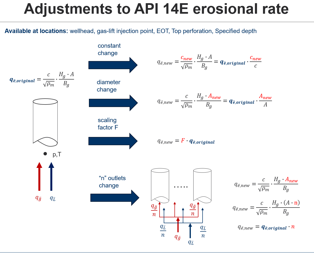
Why is the default erosional rate depth 'Wellhead'?
Within the tubing, the pressure is lowest at the Wellhead, and therefore the gas velocity is the highest. This is the location, within the tubing, we are most at risk for erosion. In short, if there is no erosion at wellhead, it is likely there won't be erosion deeper in the tubing, due to the pressure decreasing and the gas velocity speeding up. Alternatively, we may be below the erosional rate at the EOT but that tells us nothing about whether we have erosion at the wellhead.
BHP Calculation Dependency for Erosional Rate Correlation
Ensure that the BHP is calculated at least once and an appropriate 'Bottomhole Pressure to be used in calculations' is also chosen because the erosional rates will change accordingly. You need to strictly use one of the erosional models for calculating erosional rates. If you have 'Measured pwf, gauge' or 'Custom pwf' selected in 'Bottomhole Pressure to be used in calculations', they will default to Hagedorn and Brown.
Erosional Rates can be calculated for the following critical rate depth types:
| Depth Type | Description |
|---|---|
| Wellhead | Erosional rate is computed at the wellhead, i.e., at surface (depth of 0 ft). |
| Top Perforation | Erosional rate is computed at the top perforation depth (as entered in the well data card). |
| End of Tubing | Erosional rate is computed at the end of tubing, i.e., at the tubing intake (as per the wellbore configuration). |
| Minimum Rate | Erosional rate is calculated at all depths and the reported rates are the minimum rates calculated (that could be at variable depths) throughout well history. |
| Specified | Using this option, you can manually specify the fixed depth at which erosional rates are to be computed throughout well history. |
3.11.5. Why is the erosional rate under the gas lift optimization tab (Nodal) sometimes different than the erosional rate shown in the BHP module for this day?
The workflow to calculate erosional rate is to first run a BHP calculation, with the given gas (and input lift gas rate, if any). Then, at the specified location (wellhead, gas lift valve, etc.), one uses the method equation to estimate erosional velocity (depending on whether using API 14E or Svedeman and Arnold). Lastly, one converts the velocity to rate by
where is gas holdup, is cross-sectional area, and is gas volume factor.
Since these equations use fluid properties like liquid and gas density to calculate mixture density (API 14E only), liquid holdup, and gas volume factor, in principle, they depend on the pressure and temperature at the location that is an output of the BHP calculation.
Consequently, the value of the erosional rate could change (sometimes significantly, sometimes slightly) as a function of the BHP calculation input.
When the erosional location is wellhead, usually pressure and temperature are constant in time, so most inputs to the erosional rate calculation will be constant. However, the erosional rate could still vary if there are variations in GOR/GLR. GOR/GLR variations cause changes in liquid holdup, which affects the calculation of the mixture density (API 14E) and the conversion from erosional velocity to erosional rate. Variations in flowing GOR/GLR through the tubing occur with, for example, gas lift.
As an example, the figure below shows a gas lift performance curve giving oil rate versus lift gas injected. The figure also shows (in the secondary vertical axis) the values of the API 14E erosional rate at wellhead for each lift gas rate injected and the total gas rate (lift + reservoir gas) circulating through the tubing. There is significant variation of the erosional API 14E rate with lift gas rate. w+ compares the total gas rate with the erosional API 14E rate to determine if there is an erosion risk or not.
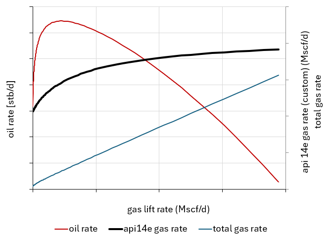
3.12. Injection of surfactants (foamers) and DRA (drag reducing agents)
3.12.1. Foamer (surfactant) injection
In some situations, for example gas wells producing with some associated oil and water, a capillary string is used to inject a foaming agent into the wellbore. This has several effects, mostly positive, such as causing gas to be entrained in the liquid and reducing the overall density. The foamer also modifies the transition between flow patterns and could cause the liquid mixture to exhibit a higher apparent viscosity.
whitson+ has an approximate method to model the effect of a foamer. The presence of a foamer can be activated (3) by clicking in the well data card (1), then further on the "fluid settings" (2).
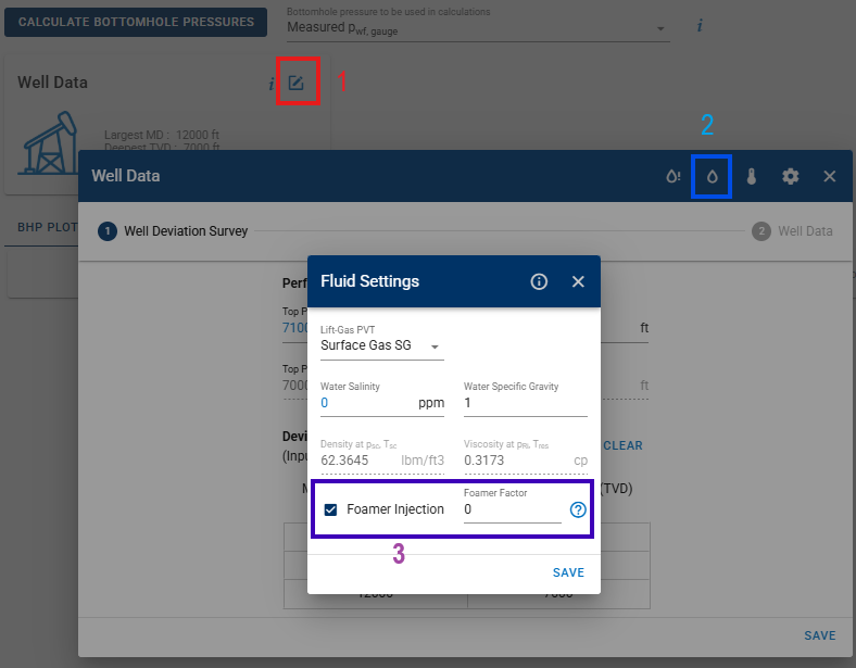
A factor between 0 and 1 can be input. A value of 1 will give no slip between gas and liquid, representing an optimal and ideal foamer homogenizing effect. A value of 0 will give the original value of the slip as given by the multiphase correlation.
Foamer applies to all multiphase correlations
The foamer factor will apply to all multiphase flow correlations, but will be ignored for all single-phase calculations.
Foamer applies to flow throughout complete wellbore
The foamer factor will apply to flow through the complete wellbore.
3.12.2. DRA (drag reducing agent) injection
Drag reducing agents are used to attempt to reduce friction losses in pipe flow by modifying the turbulent flow structures. whitson+ doesn't have a built-in method to model the injection of a drag reducing agent. As a workaround, you can use the BHP tuning factor beta to capture the effect. When on the BHP module, click on "tuning" and manually modify the friction factor correction (beta): corrected_friction_factor = original_friction_factor * beta. A beta of "1" gives you the original friction factor with no correction. "0.1" (lowest allowed value) gives you reduced friction effect.
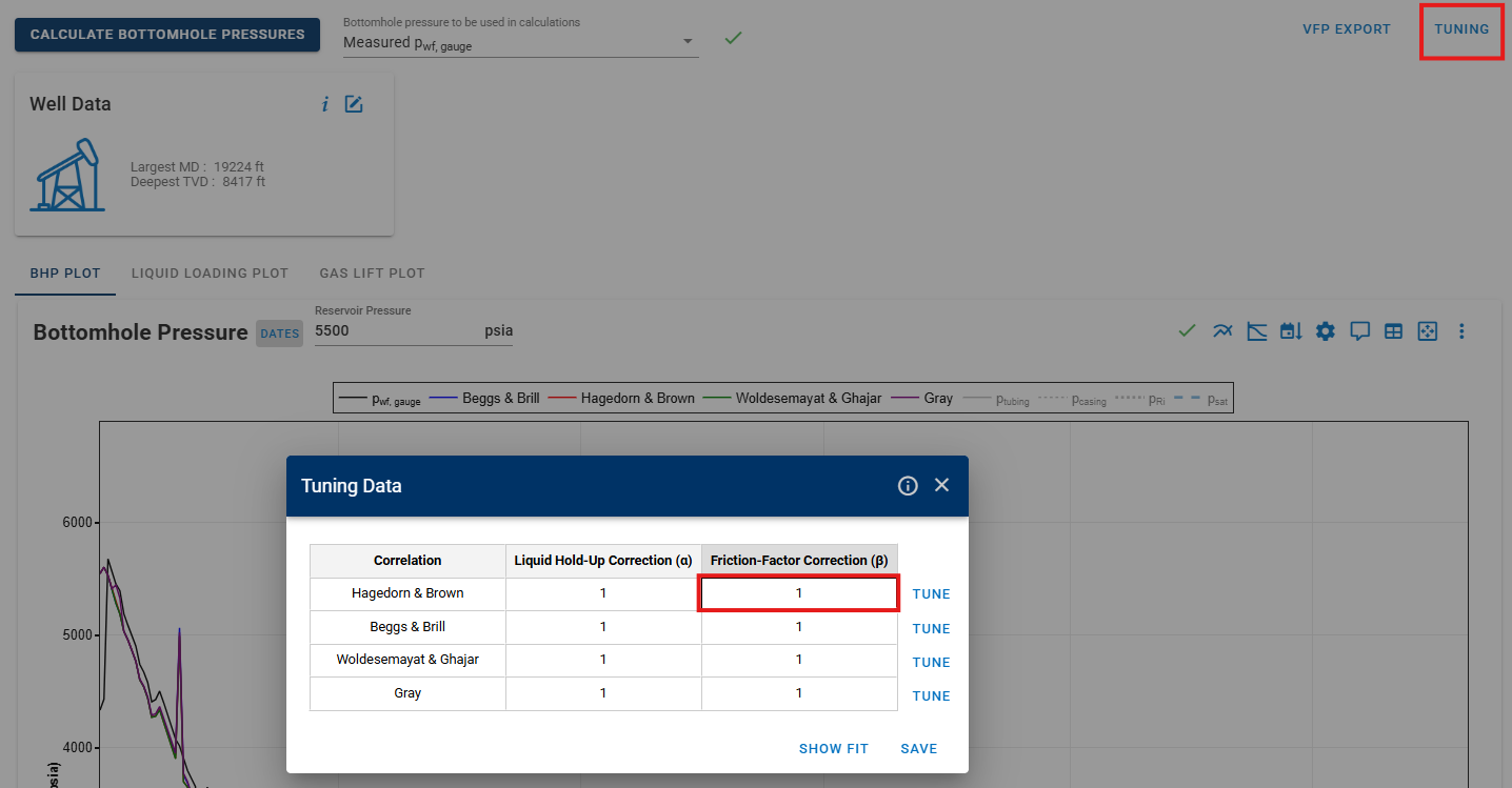
The beta factor applies to multiphase flow only
The beta factor will apply to the specific multiphase correlations, and will be ignored for all single-phase calculations.
References
[6] [H.B. Bradley, Petroleum Engineering Handbook. 3rd Edition, Society of Petroleum Engineers, Houston. 1992.]
[7] [American Petroleum Institute. Recommended practice for design and installation of offshore production platform piping systems (API RP 14E: 1991). American Petroleum Institute.]