Comparison Plot
This module can be used to create custom comparison plots for multiple analyses. All wells in the project can be plotted together for standardized reporting or analysis. The selected data can consist of raw inputs or values calculated in whitson+.
This module allows you to do the following:
- Select, create, and edit custom plots.
- Select wells to include in the plot.
- Customize traces, colors, markers, and legends.
- Save plots and data.
You can create a multi-well comparison plot by navigating to the Comparison Plot module under Multi-well Analysis.
1. Main Plot
The main plot is created by default. It is the traditional way of accessing the comparison plot.
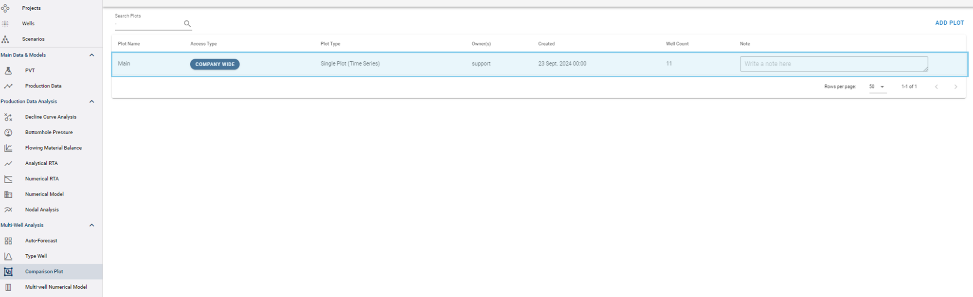
You can access previously created templates here.
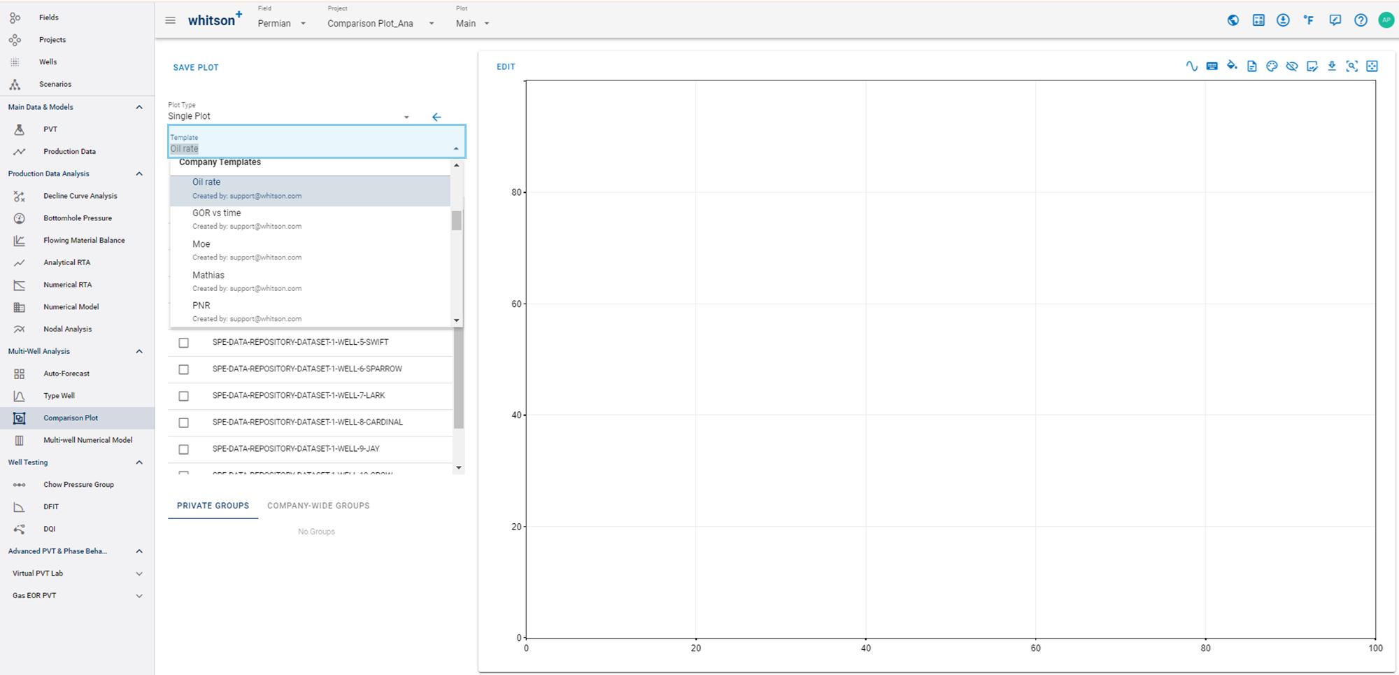
If You Want to Create a New Template
We recommend using the Add Plot option instead. This is why we removed the ability to create new templates.
You do not need to rebuild your old templates as new plots; you can continue using them as they are. However, the Add Plot option offers the advantage of saving both the well selection and layout, whereas templates save only the layout.
2. Adding Plots
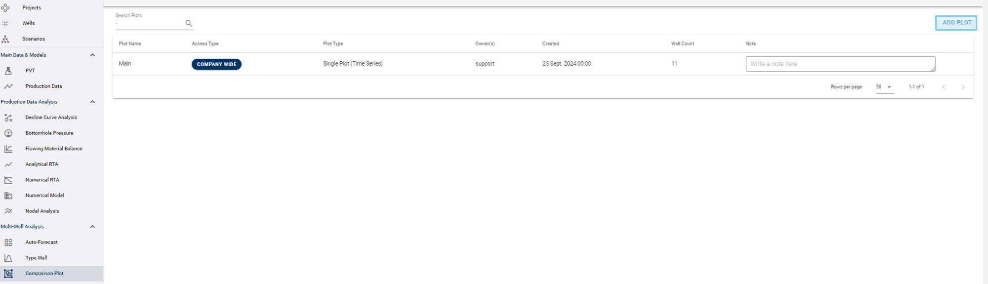
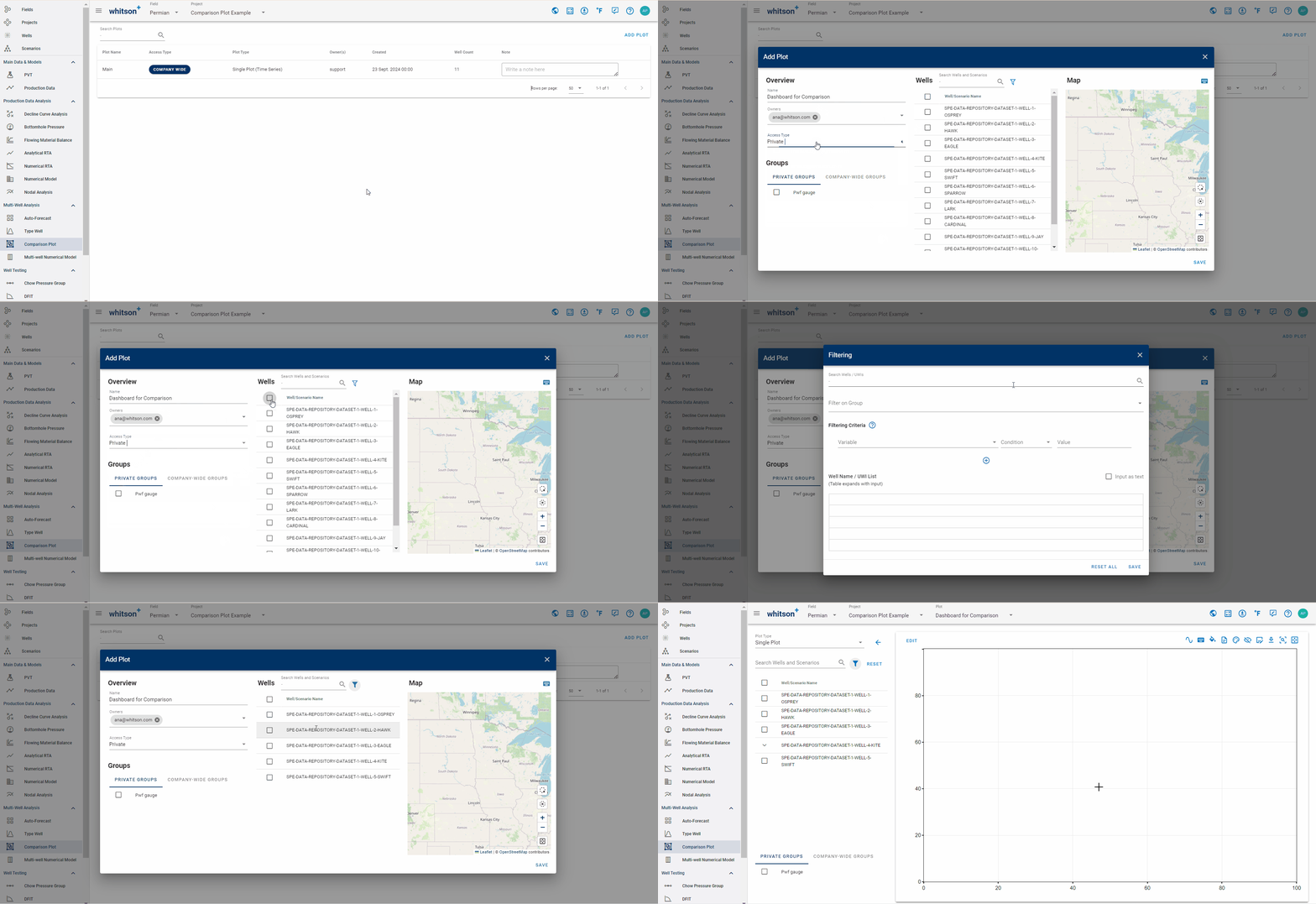
Click the Add Plot button in the upper-right corner.
2.1. General Plot Settings
2.1.1. Overview
-
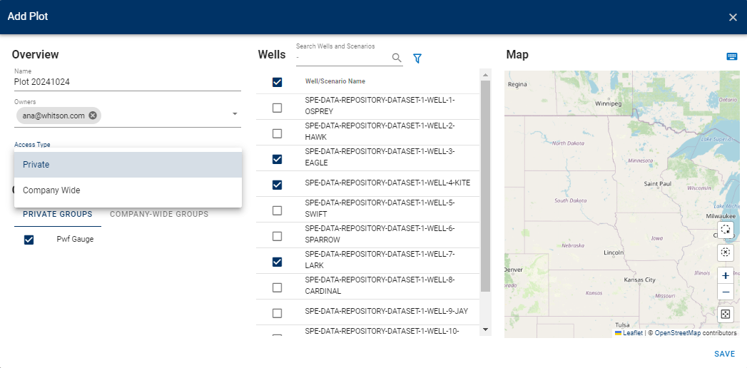
Name: Specify a name for this new plot.
-
Owners: By default, the plot owner is the person who created it, but additional people can be added as plot owners.
-
Access Type: Select the access type: private (viewable and editable only by the plot owners), company-wide (accessible to everyone in the company who has access to the software), or restricted (accessible to everyone in the project, but editable only by the owners).
2.1.2. Groups
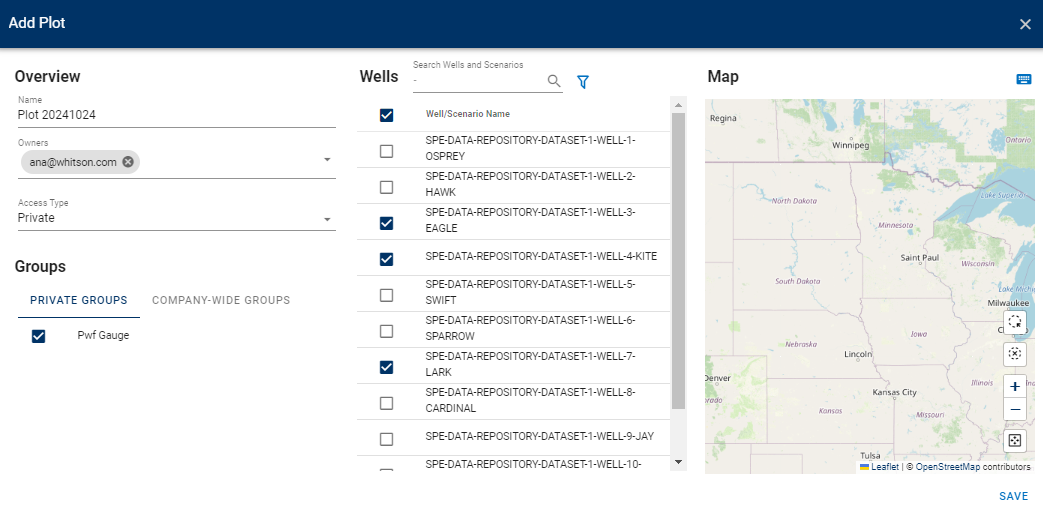
You can use pre-existing group tags to quickly identify and select the wells you want to include in your new plot.
2.1.3. Wells
There are three ways to select the wells to include in the new plot:
-
Manual: Select the checkboxes beside the well names shown in the well list.
-
Search Wells and Scenarios: Enter the name of the well or scenario, and then select the corresponding checkbox.
-
Filter Well List: Filter wells based on different criteria.
2.1.4. General Plot Editing
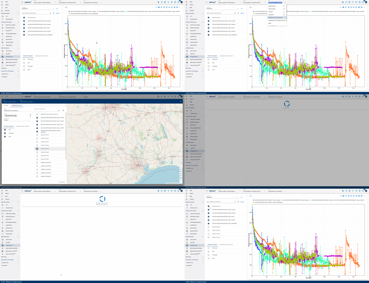
To add wells to or remove wells from the existing plot:
- At the top of the screen, open the Plot dropdown menu.
- Click the Edit Plot button.
- Select or clear the checkboxes beside the wells you want to include or exclude.
- Once the wells are selected, click EDIT PLOT.
2.2. Editing a Plot
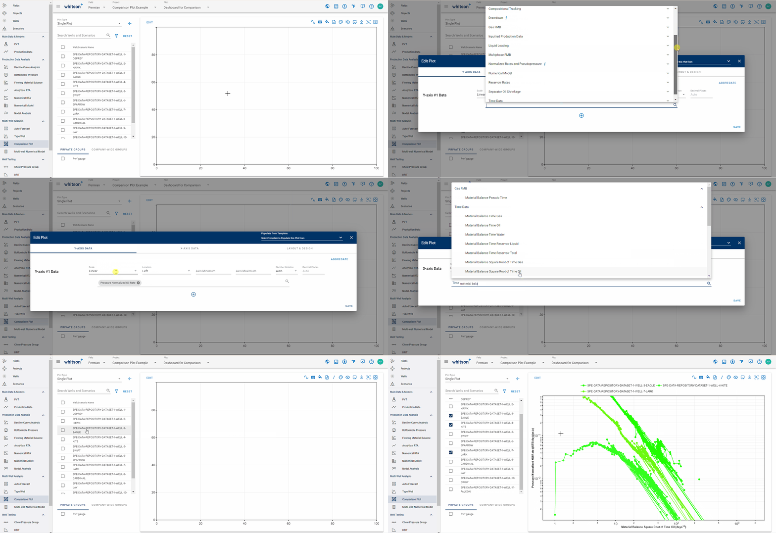
Editing a plot allows you to adjust the five main components that define the plot:
- Data plotted for each well (raw or calculated well information),
- Axis scale (linear or logarithmic),
- Axis location (left or right),
- Axis bounds (set manually or determined by the data), and
- Number notation and decimal places (Auto, Number, or Scientific).
2.3. Using Old Templates
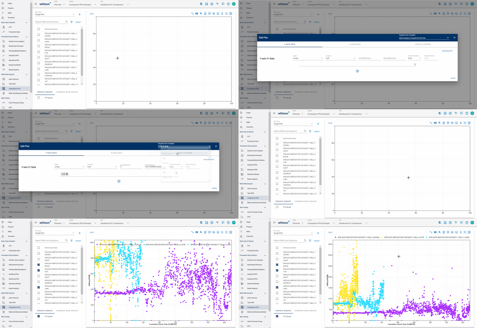
When creating a comparison plot, select Populate from Template in the upper-right corner to use an existing template as its basis.
2.4. Customizing Layout and Design
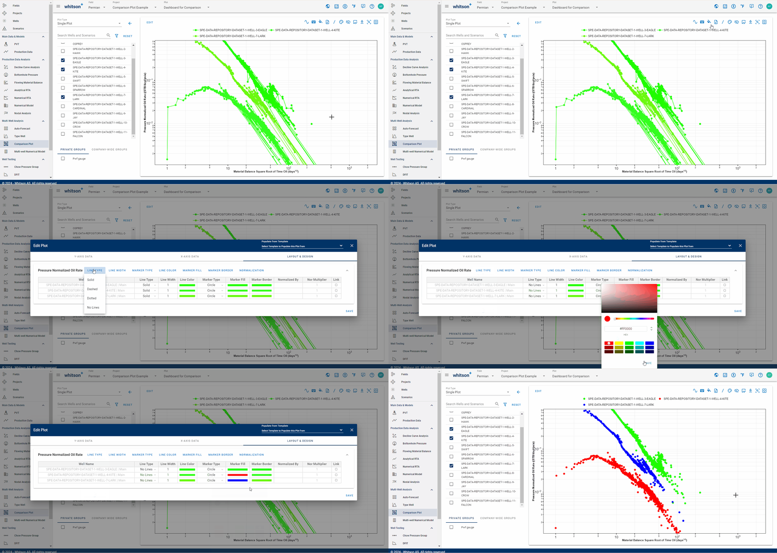
To customize the layout and design, click Open Layout and Design or Ctrl-click any plot line. You can then adjust the line type, width, color, marker fill, and marker border.
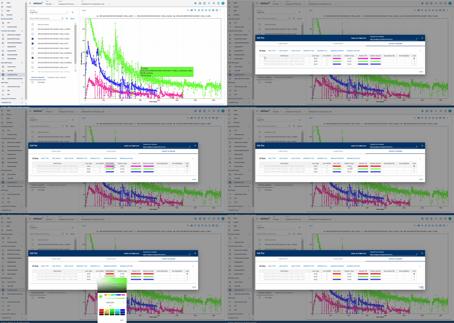
You can link the colors of all properties for a given well: line color, marker fill color, and marker border color. Once linked, changing one color automatically updates the others. If the colors are not linked, you can adjust each one independently.
2.5. Modifying the Legend
Customize the legend by clicking Change Legend.
You can select from the following options:
- Default: Shows the series name, well name, or scenario name for each data series. Clear the Default checkbox to choose the specific legend fields that best suit your needs.
-
Truncate legend:
- Truncate: Displays an abbreviated version of the legend.
- Do not truncate: Displays the full legend.
- Automatic: Automatically truncates the legend if six or more wells are plotted. Otherwise, the legend is not truncated.
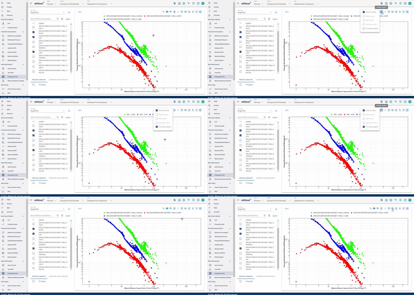
To remove the legend, click the Hide Legend eye icon in the upper-right corner.
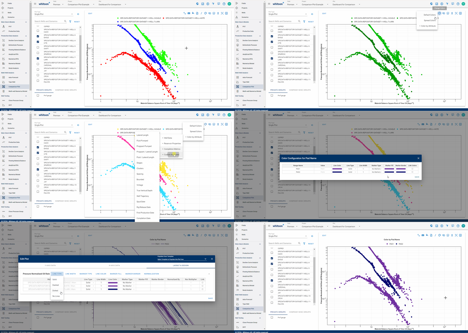
2.6. Adjusting Colors and Styles
Single Plot
You can tailor the colors of your data to your preferences using default, spread, or attribute-based schemes. Attribute-based schemes can be based on well data, reservoir properties, completion metrics, or custom attributes.
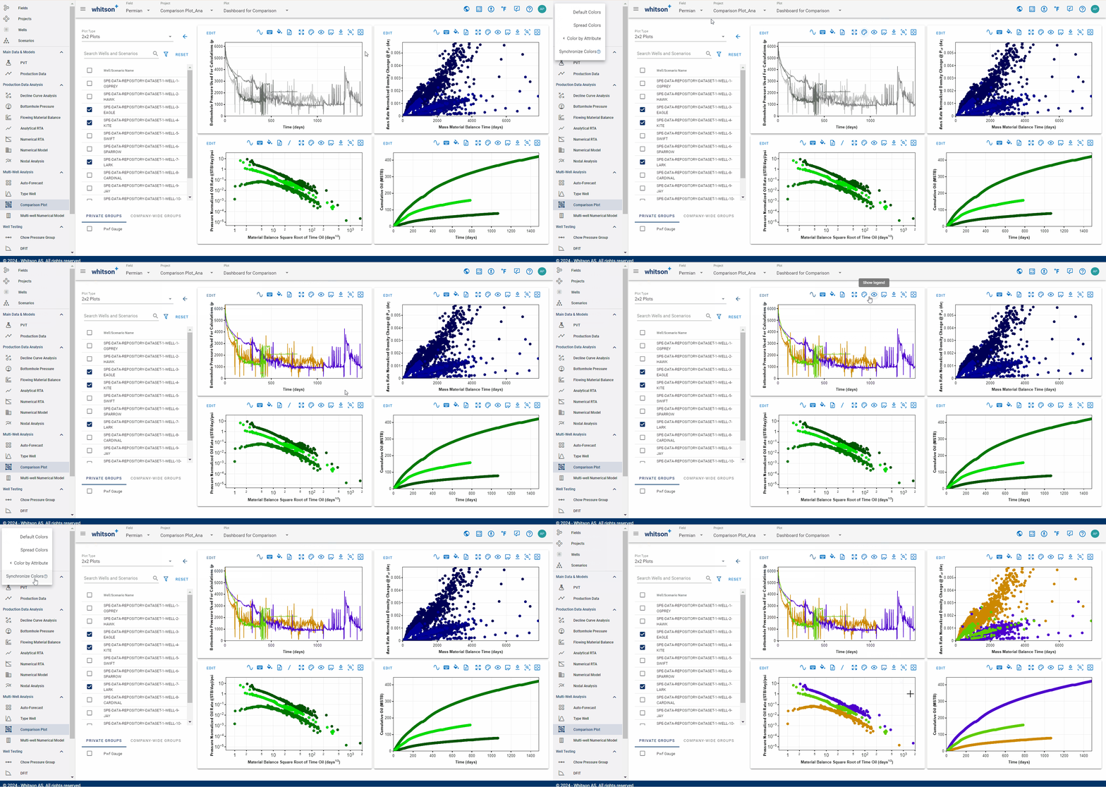
2x2 Plot
Additionally, for this type of plot, you have the option to maintain color harmony by synchronizing colors across all plots.
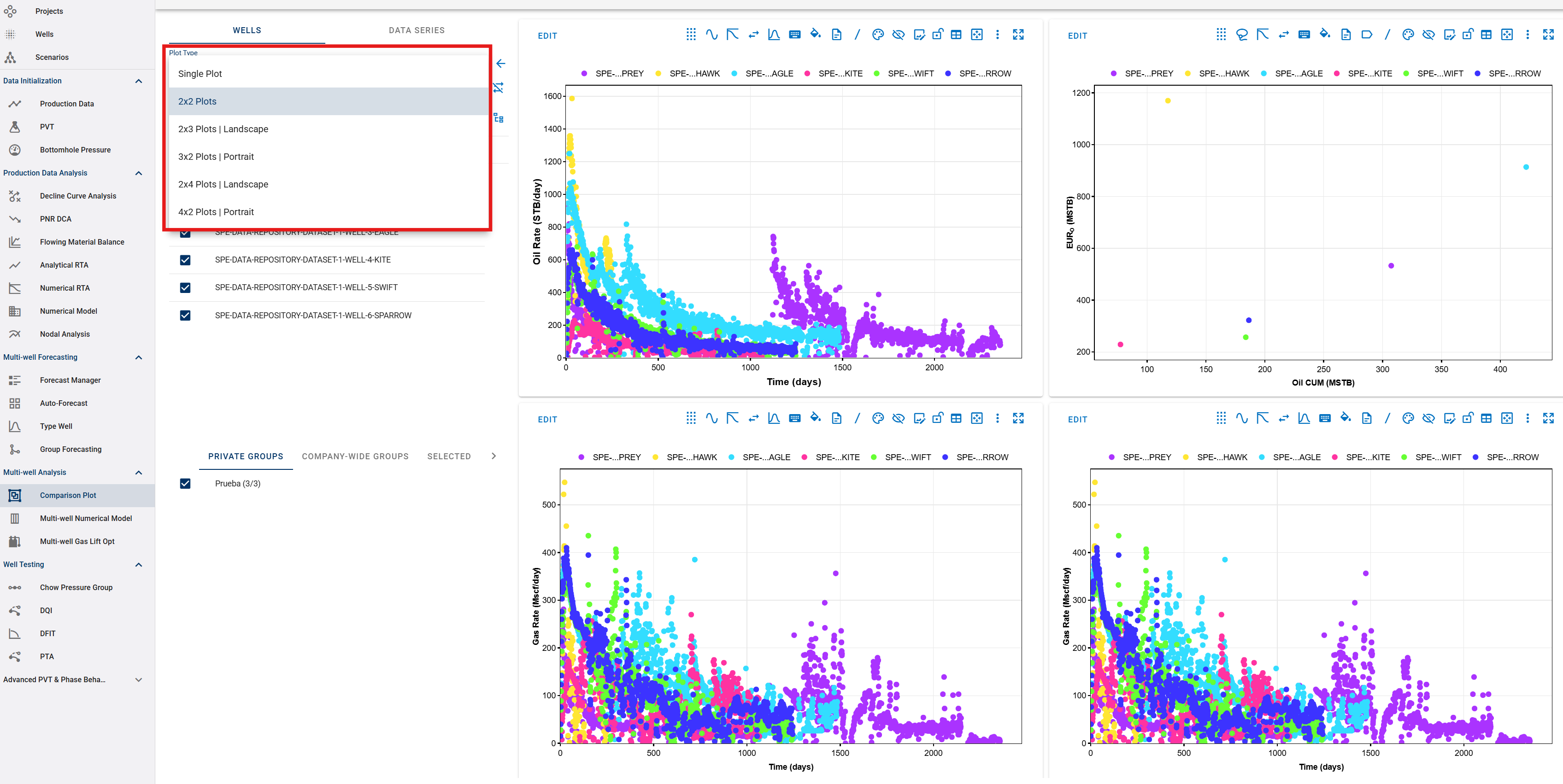
3. Single and Multi-Plot Layout
The Plot Type setting allows you to change how plots are displayed and structured on your workspace canvas. You can choose from a variety of predefined grid configurations depending on how many plots you want to compare simultaneously:
- Single Plot: Displays one full-screen plot at a time.
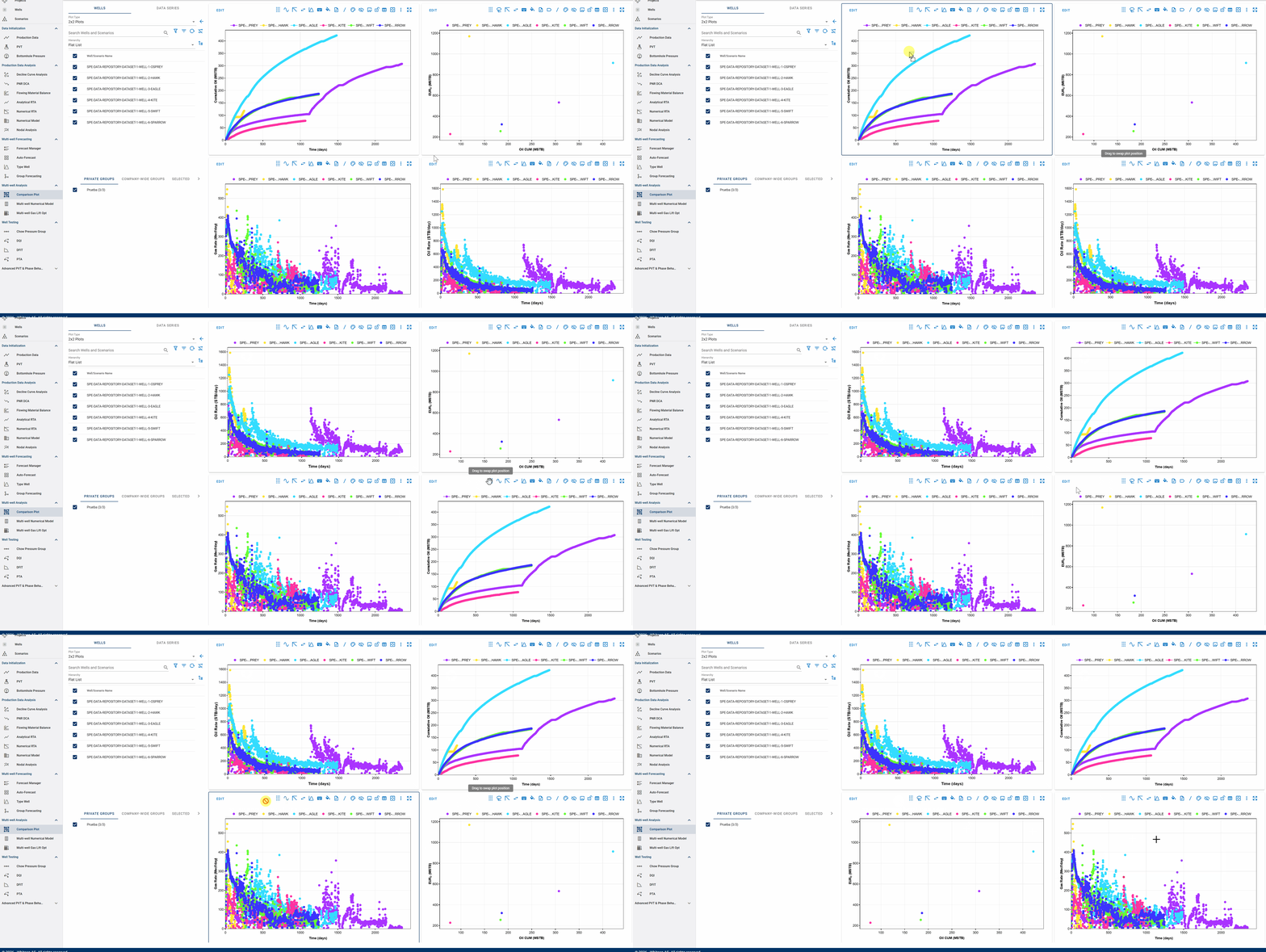
- Multi-Plot: Configurations such as 2x2, 2x3, 3x2, 2x4, and 4x2 organize your plots into structured multi-panel layouts (such as landscape or portrait orientation) to view multiple data comparisons side-by-side.
3.1. Rearranging Plots (Drag and Swap)
Once you have configured a multi-plot layout, you can easily customize the arrangement of your panels on the fly:
- Drag to Swap Plot Position: Click and drag any plot onto another plot's position to instantly swap their locations on the grid canvas, allowing you to organize your comparison views effortlessly.
4. Customizing Plot Appearance
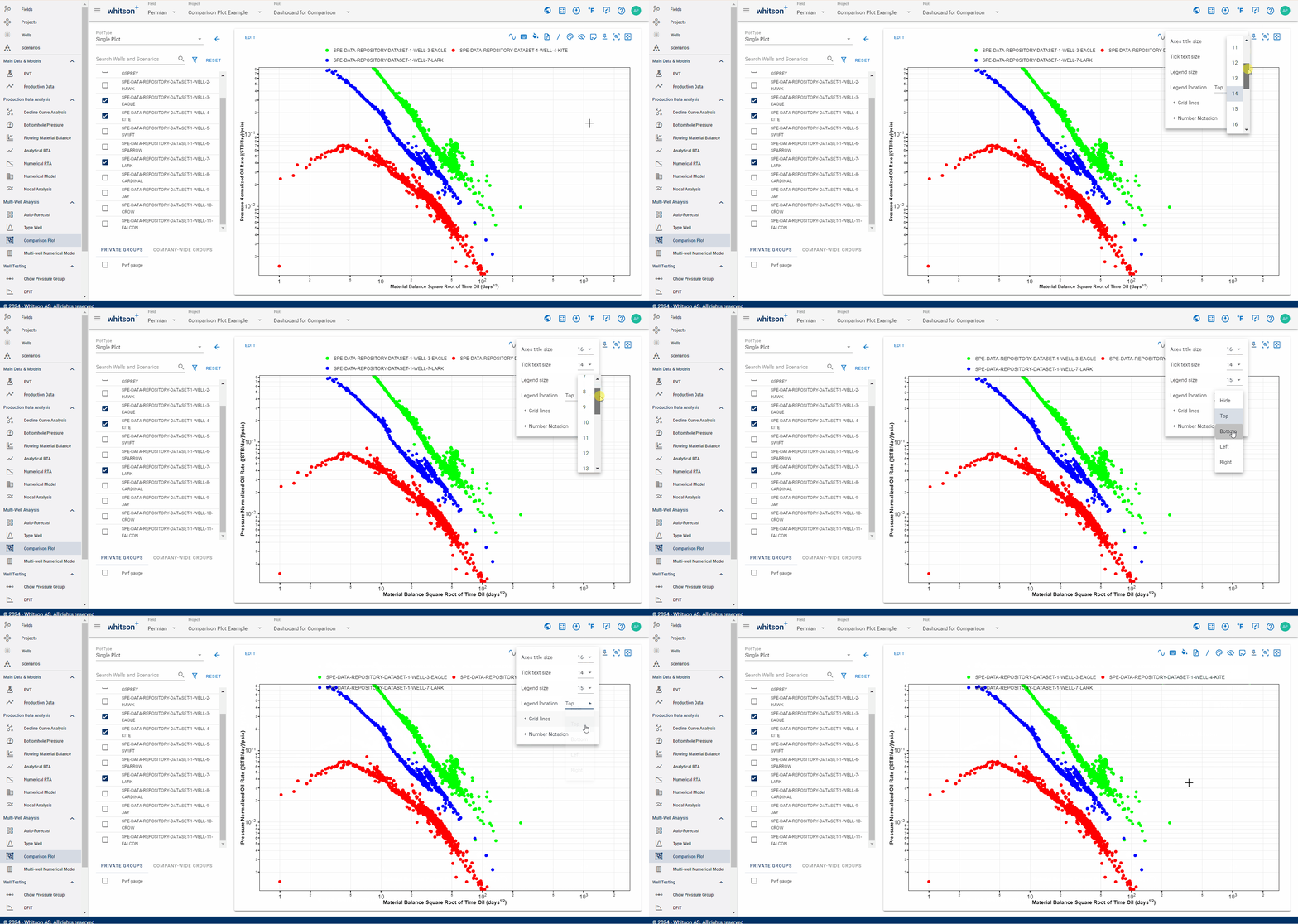
You can customize the axis-title size, tick-text size, legend size, legend location, grid lines, and number notation by clicking Customize Plot.
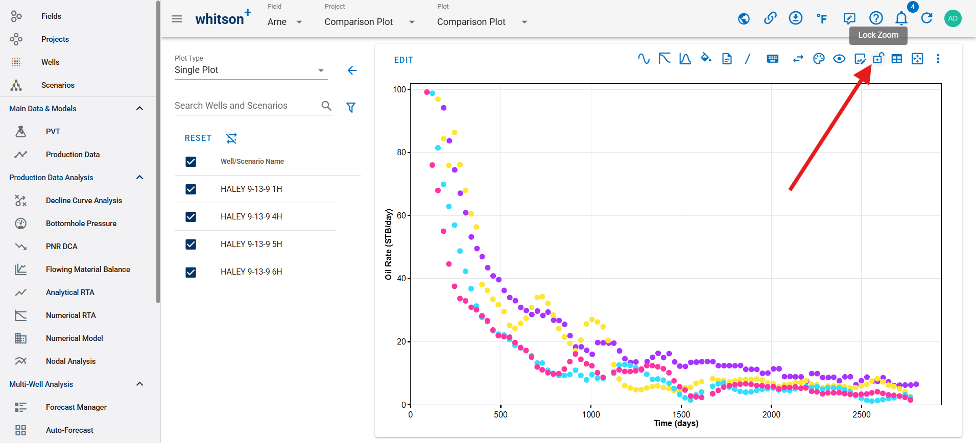
Axis zoom scales can be locked to preserve the current zoom level when interacting with the plot or refreshing the view.
5. Smoothing Data
Data smoothing can be applied to the plot by clicking the Smoothing icon. You can choose to smooth individual data series (or wells) or all data simultaneously. The smoothing function calculates a moving average across data points, which helps reduce short-term fluctuations and highlight overall behavior.
The smoothing number determines how many forward-looking data points are included when calculating the average. A higher number produces a smoother curve by averaging over a larger window, making long-term trends easier to observe and compare across wells.
Smoothing is especially helpful when working with jagged rate-time data, improving clarity and making well-to-well comparisons more effective.
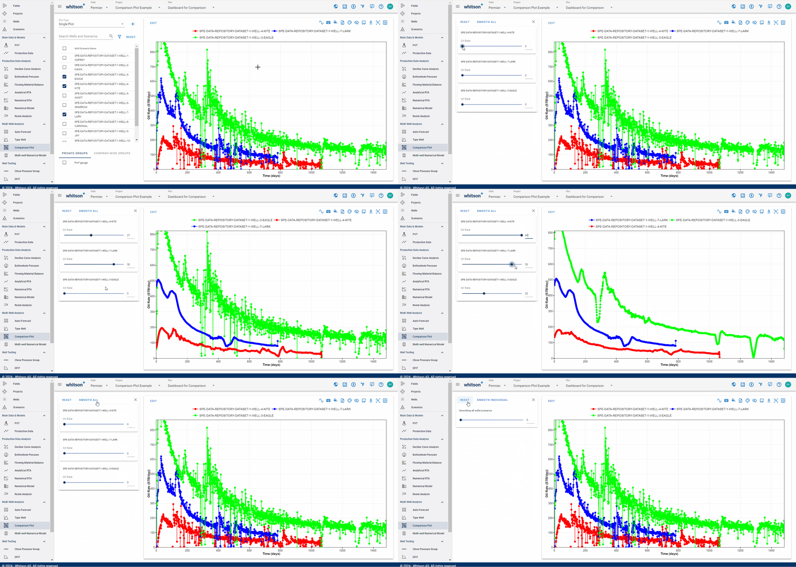
Click RESET to remove the smoothing applied to all data series.
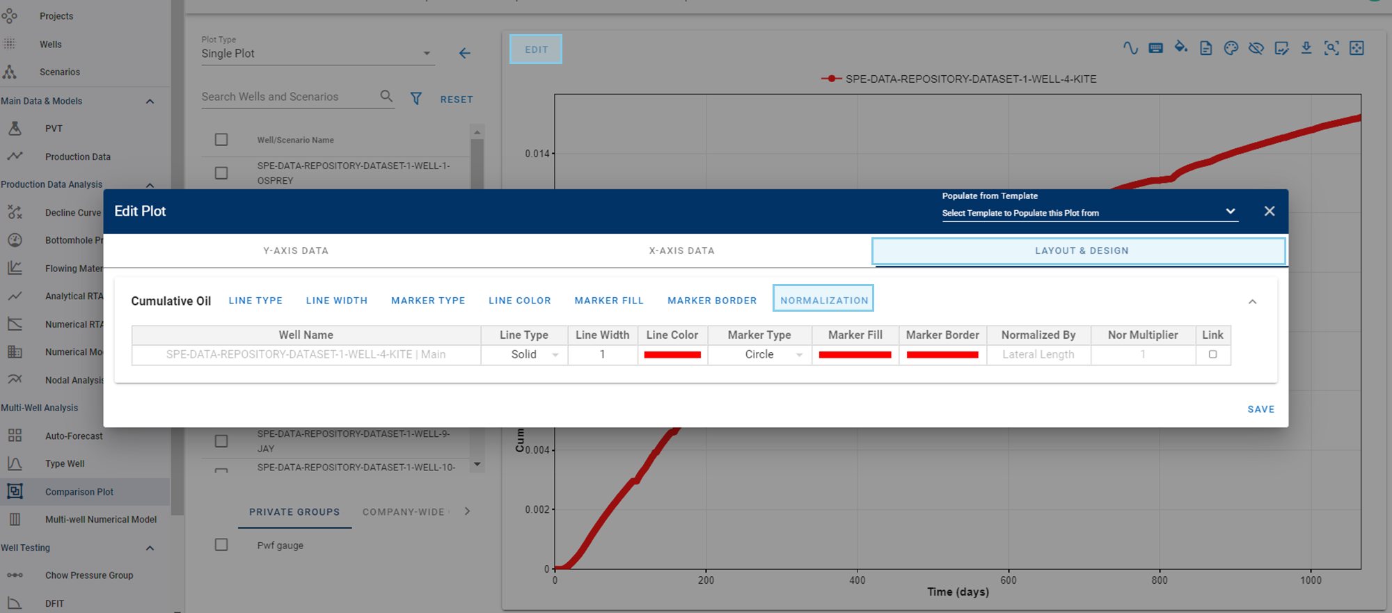
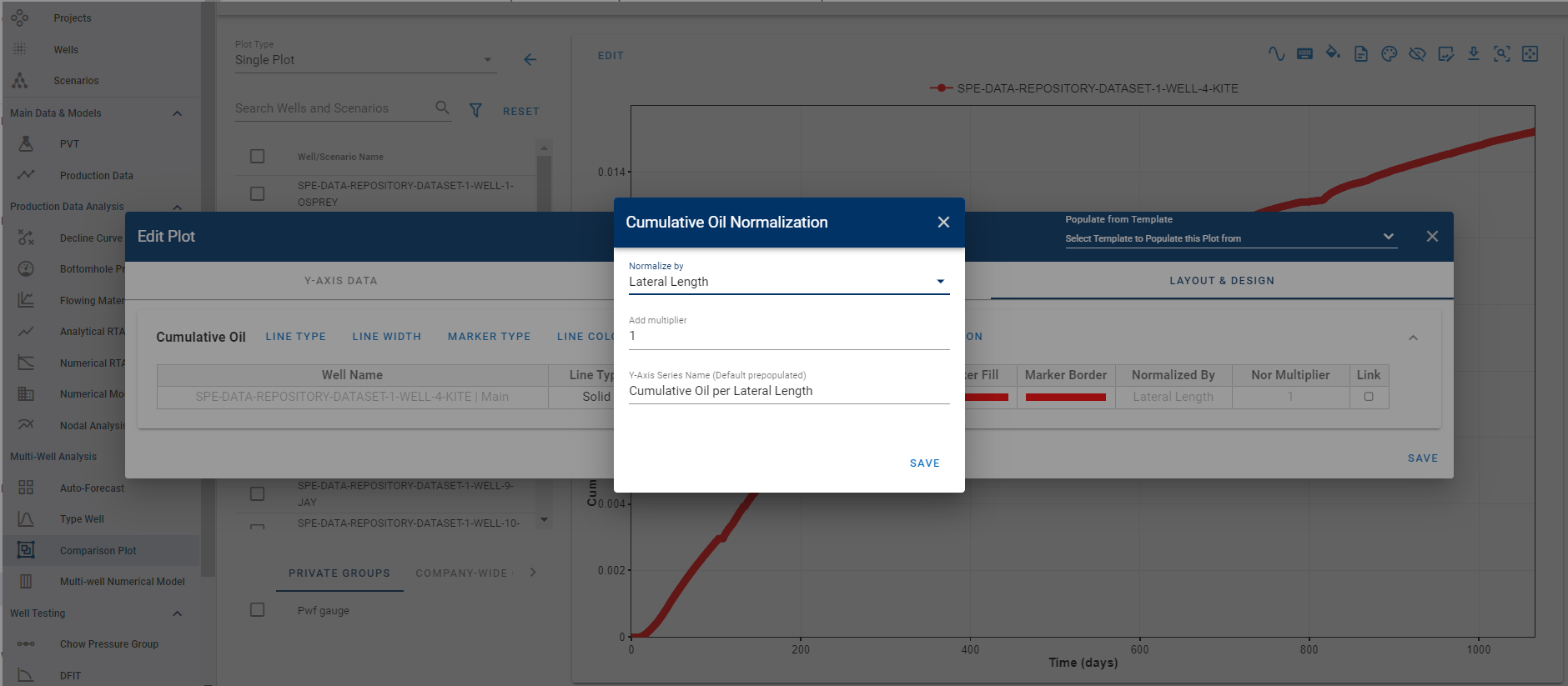
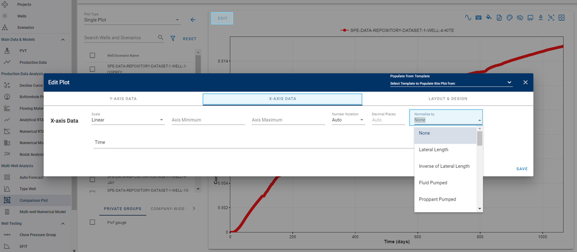
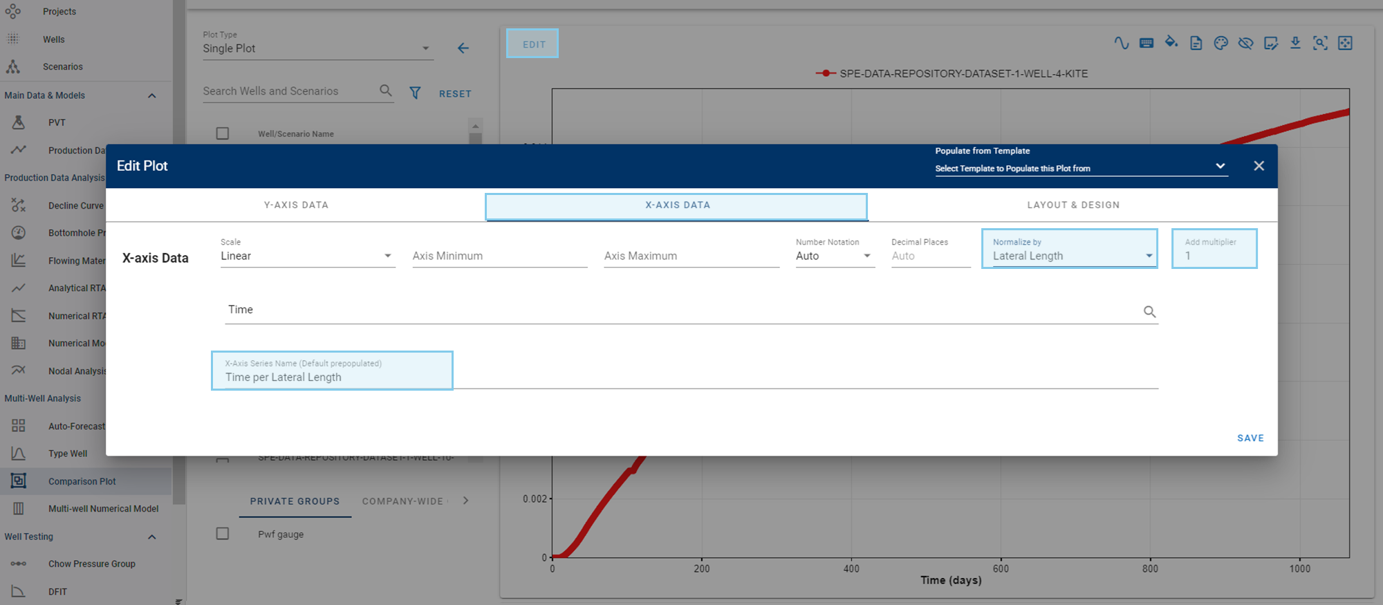
6. Normalizing Data
Both axes can be normalized by various factors, including lateral length, inverse of lateral length, fluid pumped, proppant pumped, stages, clusters, spacing, bounded, vintage, TVD, spud date, rig release date, first production date, completion date, company, pi, tres, reservoir height, fracture height, porosity, number of fractures, initial water saturation, rock compressibility, matrix gamma, fracture gamma, and water salinity.
To normalize the Y-axis:
- Click Edit.
- Select Layout & Design.
-
Select Normalization.
-
Select the normalization factor, add a multiplier, and optionally edit the series name.
-
Click Save.
To normalize the X-axis:
- Click Edit.
- Select X-Axis Data.
-
Select Normalize By.
-
Select the normalization factor, add a multiplier, and optionally edit the series name.
-
Click Save.
You may combine these two methods if the goal is to normalize both axes simultaneously.
7. Aggregating Data
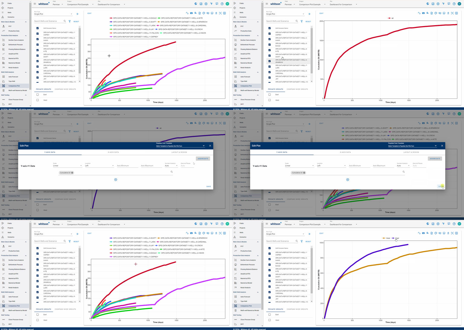
This feature generates one curve for each selected dataset by aggregating all wells. You can choose to aggregate data to view information at different levels of detail:
- All: Group data from all selected wells in the plot.
- Attribute: Group data based on specific attributes, such as company, pad name, or well trajectory.
- Group: Group data based on predefined groups, such as private or company-wide groups.
The aggregation method can be selected from the following options:
- Sum: Used for all series except pressures, which are always averaged. For series that are fractions of rates and pressures (PNR, RNP), the rates are summed while the pressures are averaged.
- Average: Recommended for pressures.
- P10
- P50
- P90
- Geometric Mean
- Swanson Mean
P10/P50/P90 Calculation in Comparison Plot
At each time step, the available values are sorted in ascending order and indexed from through . P10, P50, and P90 use the petroleum exceedance convention; therefore, P10 represents a high case and corresponds to the 90th percentile of the sorted values.
Here, is the exceedance probability (10, 50, or 90), is the number of values at that time step, and is the largest integer less than or equal to . The result is linearly interpolated between the adjacent zero-indexed values and .
The following GIF demonstrates how to use these aggregation options and methods:
8. Copying a Plot
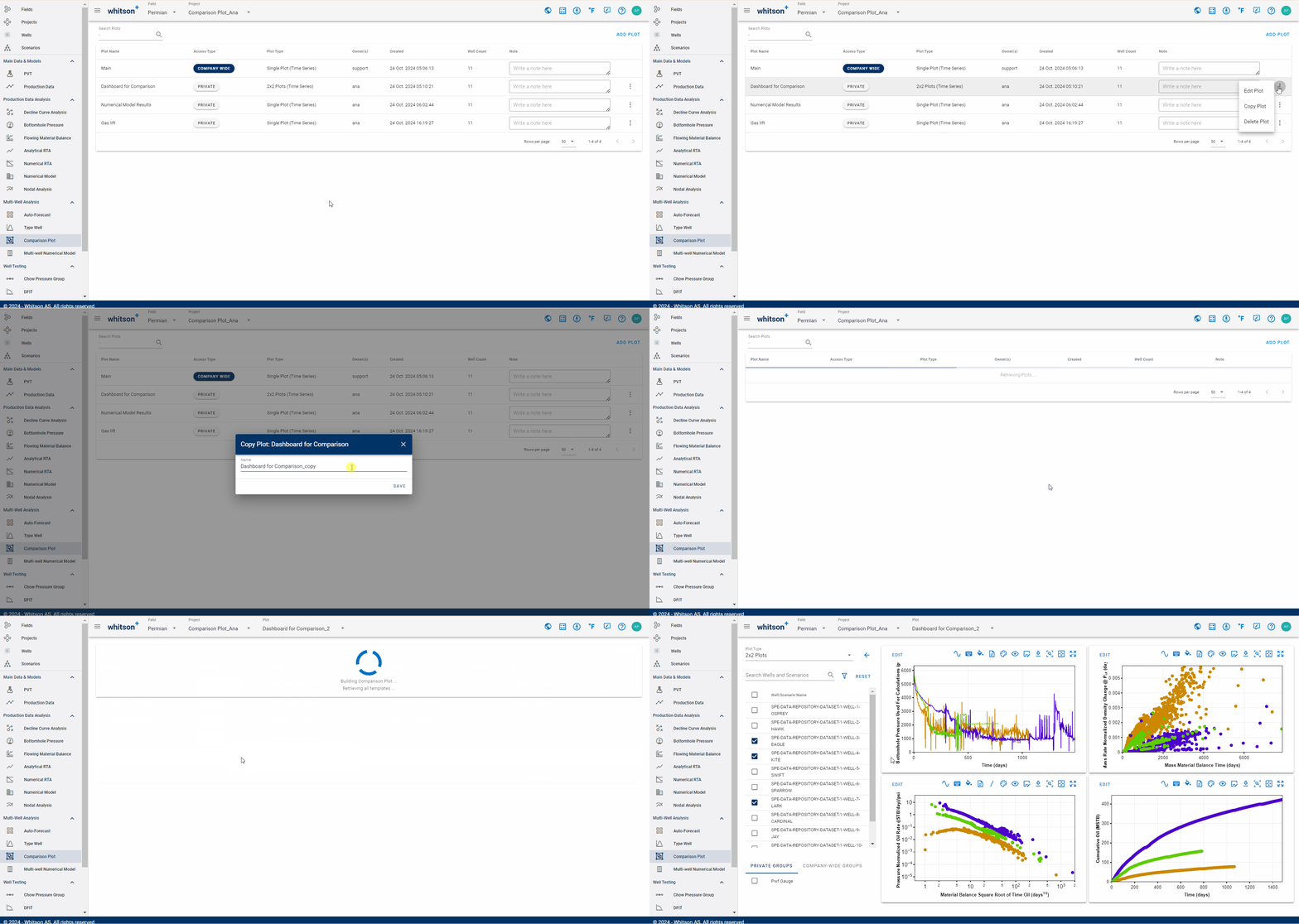
To copy a plot, navigate to the main Comparison Plot page. Locate the plot you want to copy and click the three-dot menu to its right. Select Copy Plot from the dropdown menu and provide a name for the new plot.
9. Cross Plot
The Cross Plot is another visualization feature within the Comparison Plot module that enables users to plot any two variables against each other rather than plotting time-series data. It is ideal for identifying correlations, trends, and outliers across wells or datasets without the influence of time.
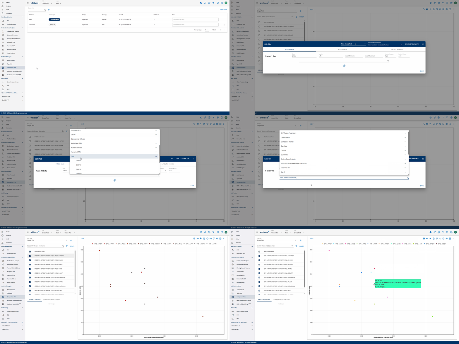
The Cross Plot functionality is available within any existing or new Comparison Plot. To activate the Cross Plot view, toggle the Cross Plot switch in the EDIT header.
9.1. Switching to Cross Plot Mode
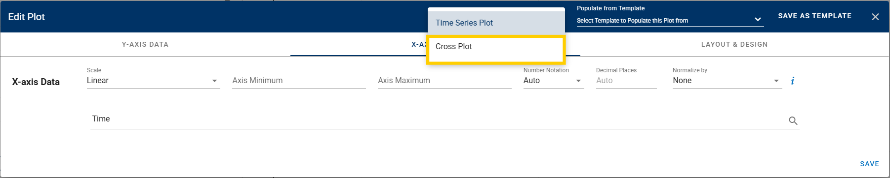
To switch a default time-series plot into a cross plot:
- Navigate to the Edit Plot window.
- Select Cross Plot in the header.
9.2. Cross Plot Features
All applicable features available in time-series plots, as described in previous sections, also apply to cross plots, including:
- Axes normalization
- Layout and appearance (marker and color settings, legend formatting, etc.)
- 2x2 plot type, multiple axis variables, etc.
You can also use attribute-based color and link color schemes to distinguish wells by operator, reservoir, or other custom attributes.
9.3. Data Labeling
The Data Labeling feature allows users to display information directly below each data point on the plot, improving interpretability and presentation clarity. Users can choose which labels appear on the plot: series name, well name, scenario name, x-value, and y-value.
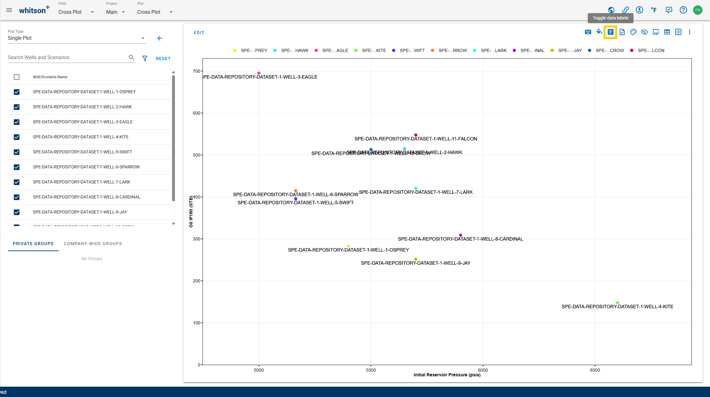
Data labeling is especially useful when:
- Highlighting outliers or key wells in presentations.
- Reviewing performance trends in relation to completion or reservoir attributes.
- Quickly identifying which data point corresponds to which well or group.
9.4. Customize by Attributes
Map both color and shape to highlight trends and categories in the cross plot.
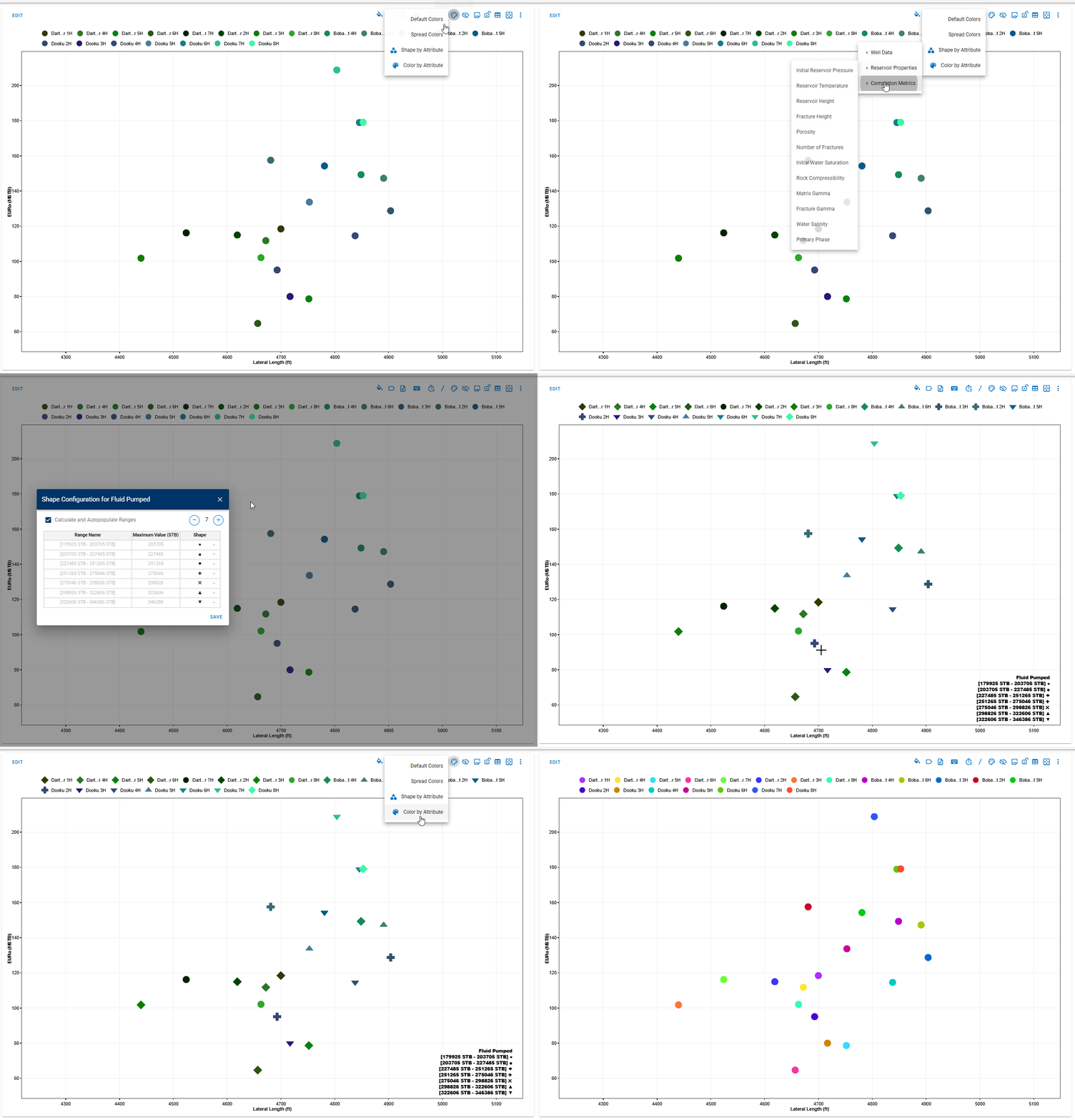
- Select the Change Colors option from the menu above the graph.
- If you haven't already, select Spread Colors to differentiate between data points.
- Scroll down to Shape by Attribute or Color by Attribute.
- For each mapping, choose the attribute that controls point shape and color.
- All steps are shown above.
10. Statistical and Category-Based Plots
In addition to time-series plots, cross plots, and GIS maps, the Comparison Plot module supports Bar Chart, Probit Chart, and CDF Chart views. These plot types can be selected from the Plot Type dropdown menu.
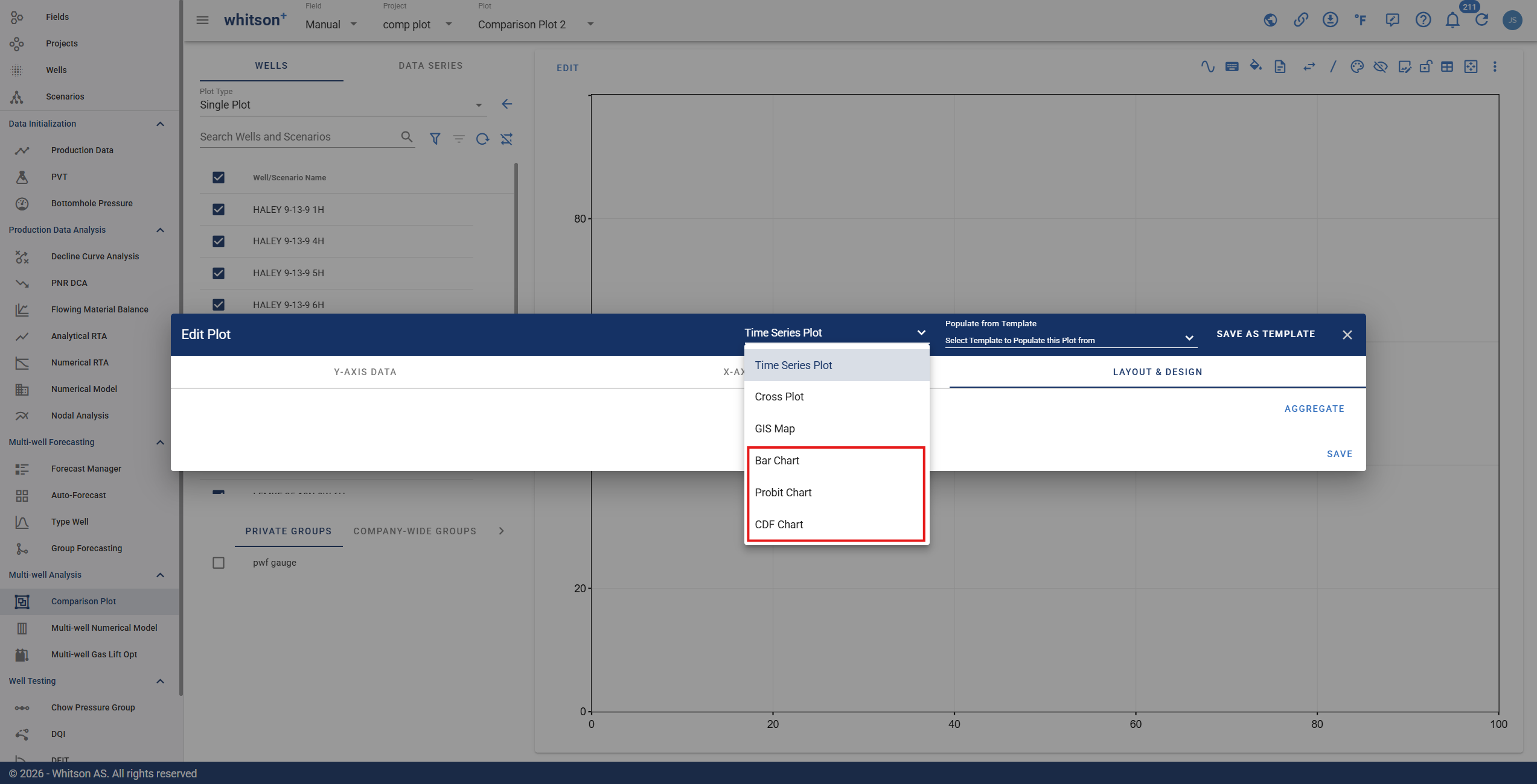
10.1. Bar Chart
The Bar Chart displays selected values as individual bars, making it useful for comparing discrete results across wells, scenarios, groups, or attributes.
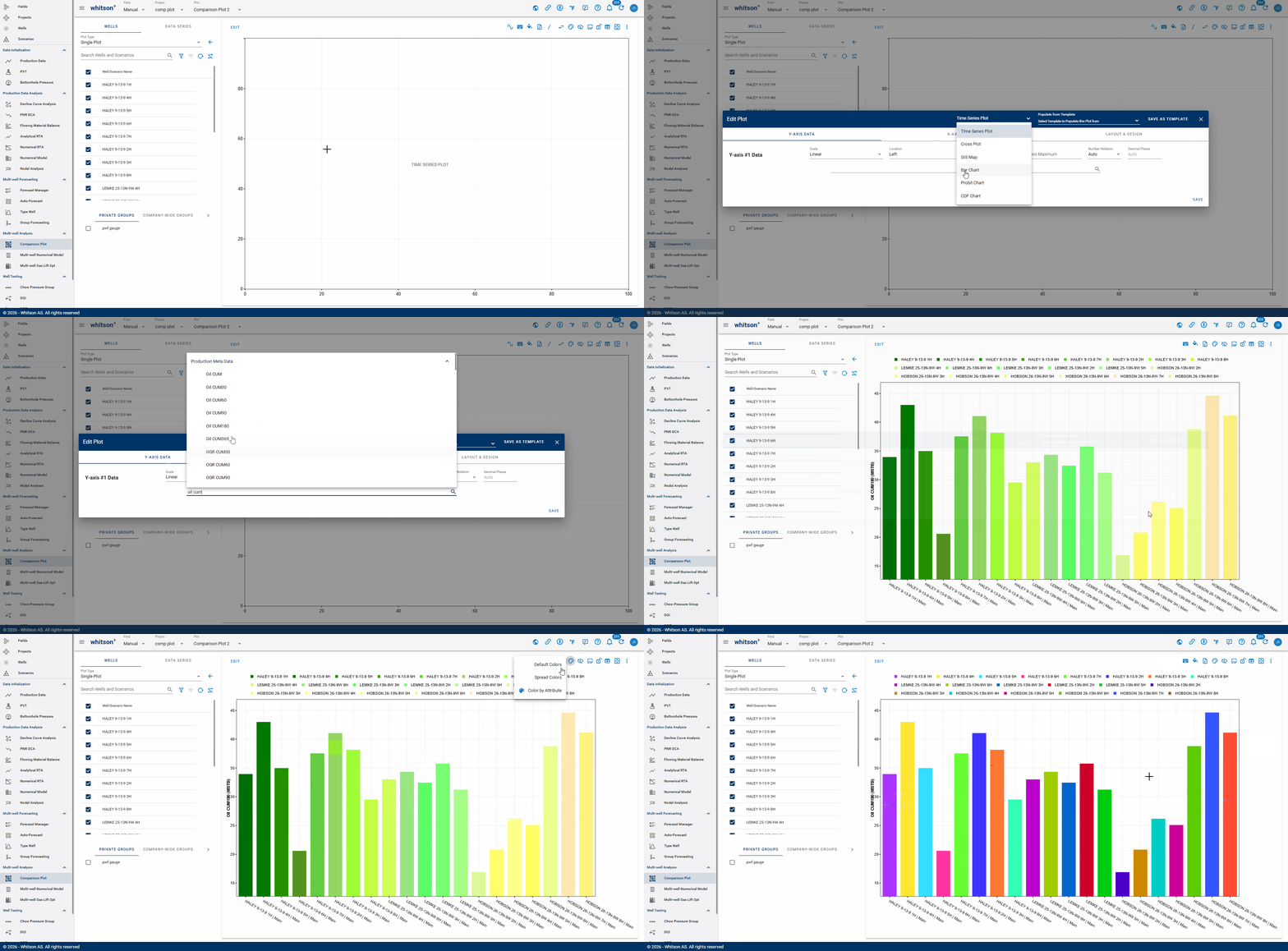
Bar charts are especially helpful when:
- Comparing a single metric across multiple wells.
- Ranking wells by production, completion, reservoir, or calculated results.
- Comparing aggregated values across groups or categories.
- Presenting results where the relative difference between values is more important than changes over time.
10.2. Probit Chart
The Probit Chart displays the selected data using a probability scale. It is useful for evaluating the statistical distribution of results and comparing datasets across wells or groups.
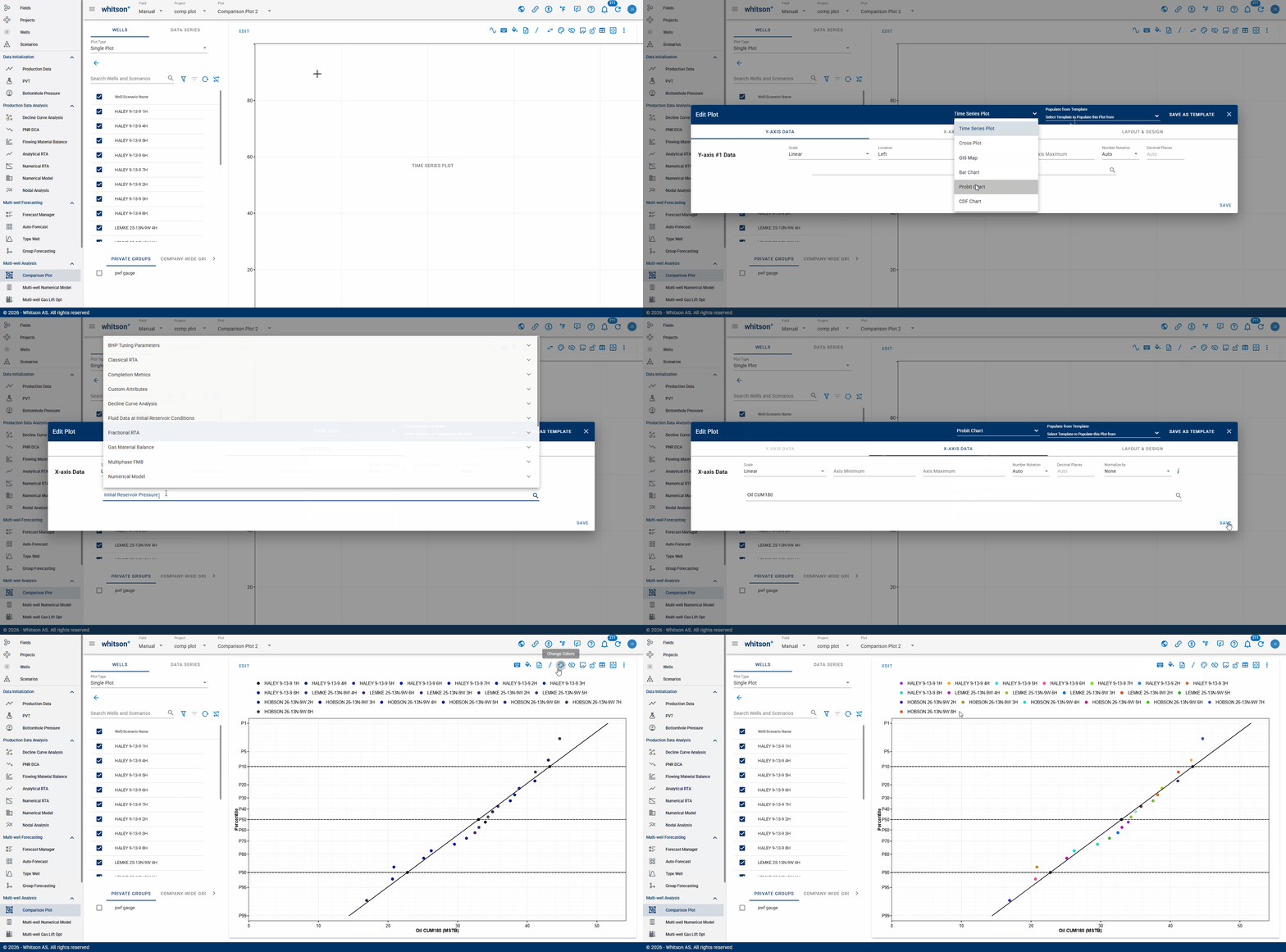
Probit charts can help users:
- Identify whether data follow a consistent statistical trend.
- Compare the distributions of different well groups.
- Identify outliers or changes in the underlying population.
- Evaluate probabilistic performance ranges.
10.3. CDF Chart
The CDF Chart, or cumulative distribution function chart, shows the cumulative proportion of observations that are less than or equal to a selected value.
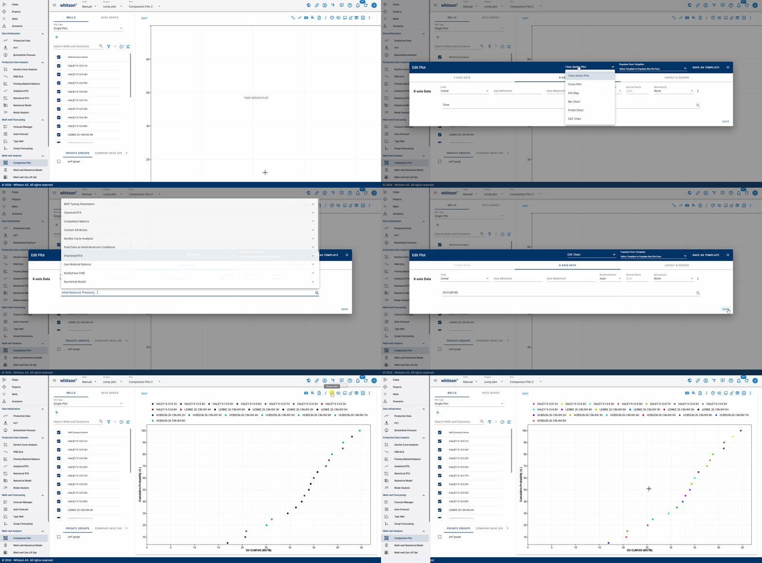
This plot type is useful for:
- Comparing the distributions of performance metrics across wells.
- Identifying percentile-based outcomes.
- Evaluating the probability that a result will fall above or below a specified value.
- Comparing uncertainty and variability between groups or datasets.
The CDF increases from 0% to 100% as the selected value increases. A steeper curve indicates that the data are concentrated within a narrower range, while a flatter curve indicates greater variability.
10.4. Hall Plot
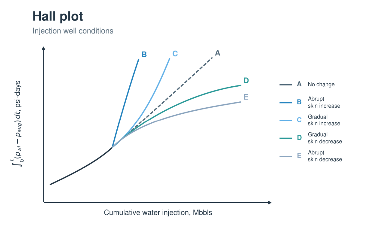
The Hall plot helps monitor injection well performance by plotting the cumulative pressure difference between bottomhole injection pressure and reservoir pressure, integrated over time, against cumulative injected volume.
- Constant slope: Stable injectivity.
- Increasing slope: Declining injectivity, potentially caused by plugging or formation damage.
- Decreasing slope: Improving injectivity, potentially caused by stimulation or fracture growth.
Interpret slope changes alongside injection history and reservoir pressure, as changes in reservoir conditions can also affect the trend.
11. GIS Map
The GIS Map feature provides a spatial visualization of wells within the comparison view. This plot type displays well locations on a map, enabling users to assess spatial relationships, patterns, and proximity between wells. The GIS Map enhances comparison workflows by adding geographical context to the plotted data.
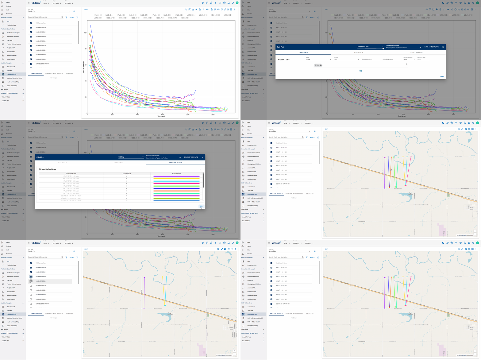
11.1. Tools
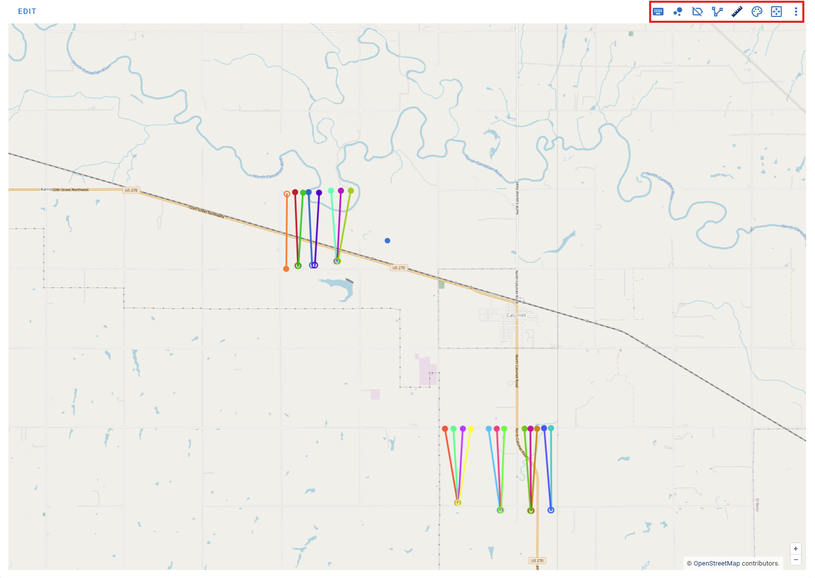
Most of these tools are also available in the software's main GIS Map. Some of the most useful tools are described below:
-
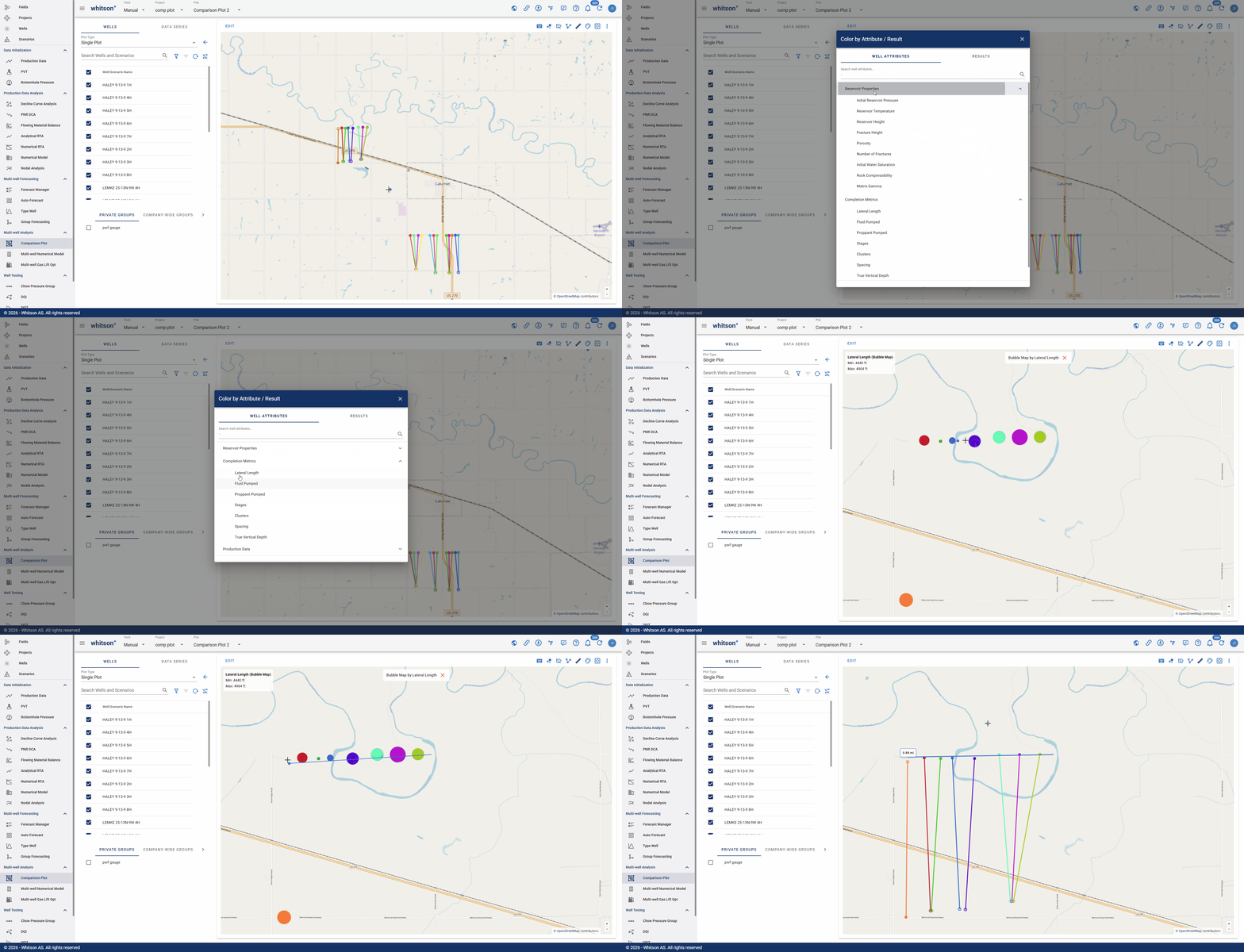
Generate Spatial Map: The spatial map can be colored by either well attributes or results to help visualize trends across wells geographically. Users can select from grouped well attributes, such as reservoir properties, completion metrics, and production data, or from calculated results, such as DCA, RTA, material balance, fluid data, and liquid loading outputs.
-
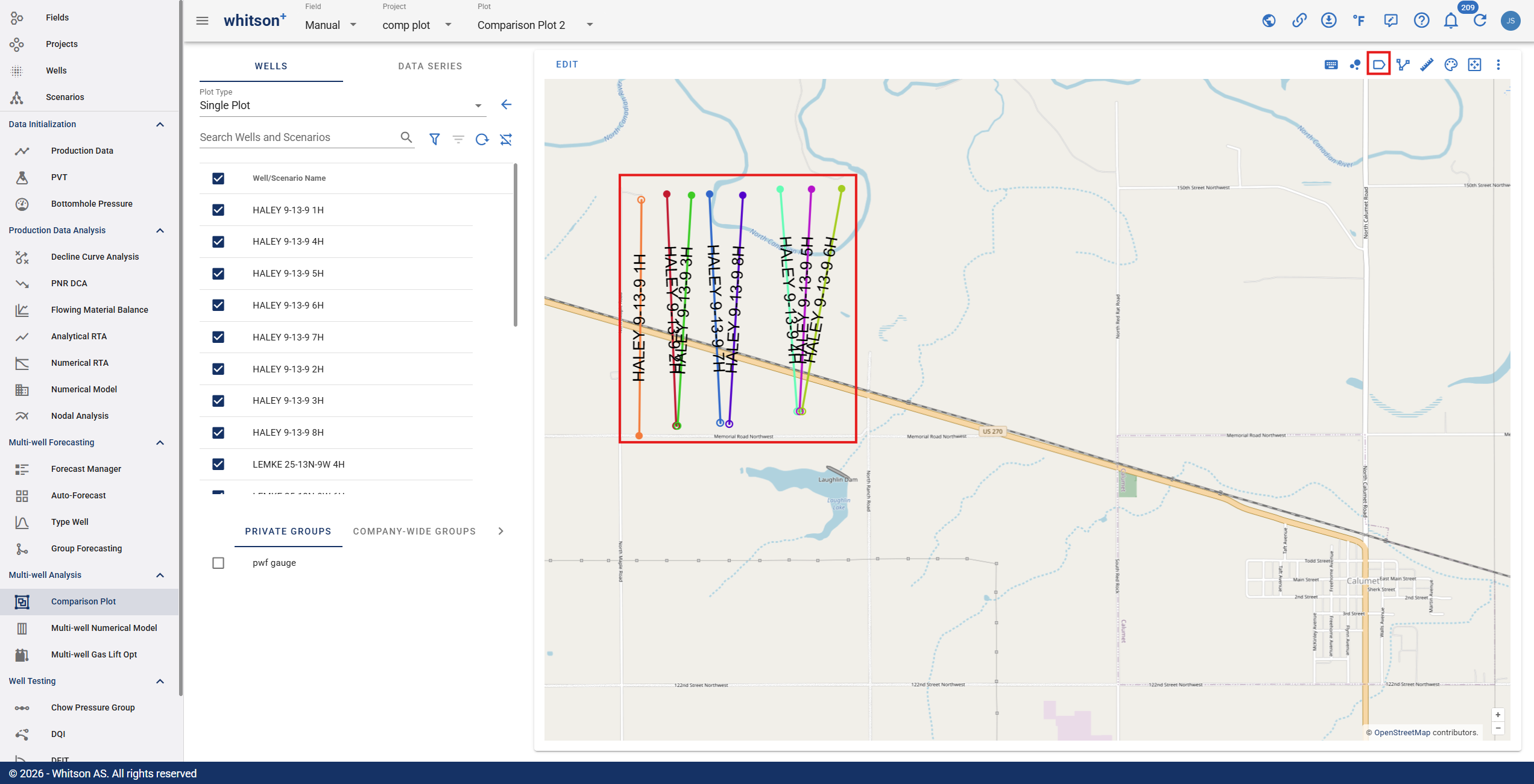
Show Well Names: Toggle on to display well names on the GIS map as labels.
-
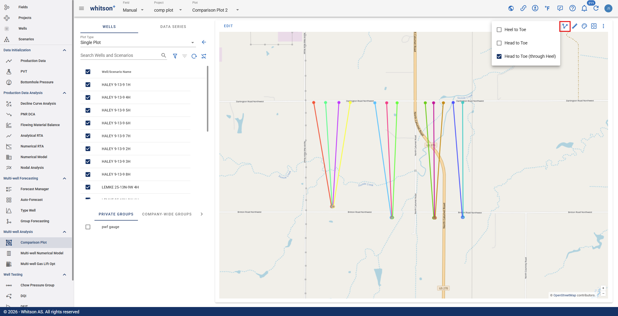
Line Type: Controls how well trajectories are displayed on the map. Users can choose between Heel to Toe, Head to Toe, or Head to Toe through Heel.
-
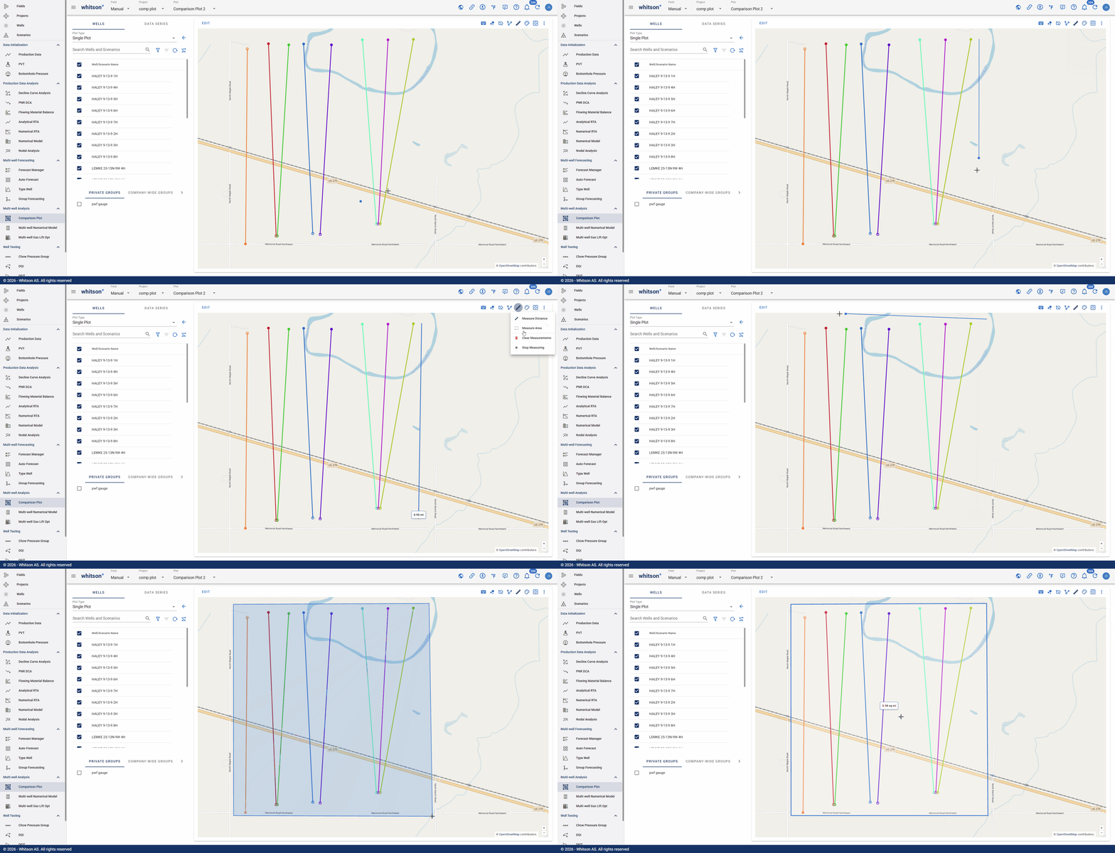
Measurement Tools: Measure the distance between two points on the map, or define a perimeter by placing multiple points and calculate the enclosed area.
12. Tips
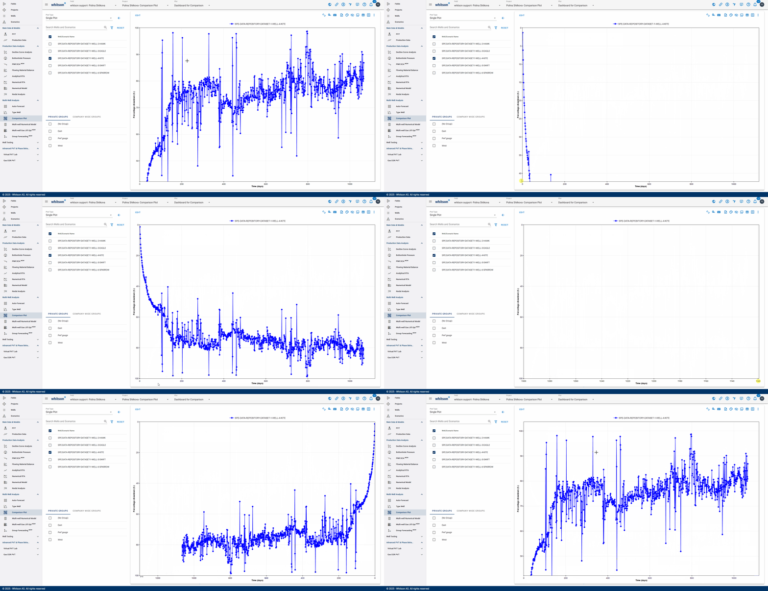
12.1. Reversing the Axis Scale
Click the minimum and maximum values of the axis you want to reverse and enter the desired values.
12.2. Using Highlighting to Elevate Your Plot
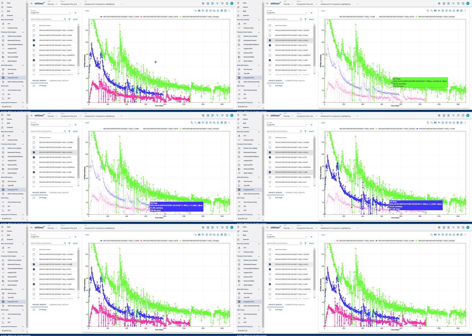
The highlighting feature can be used in a plot to emphasize a specific time series while fading the others into the background.
To highlight (or unhighlight) a time series, simply left-click it on the plot or select it from the well list. You can also click Remove All Highlights to restore the plot to its default view. See the GIF below.
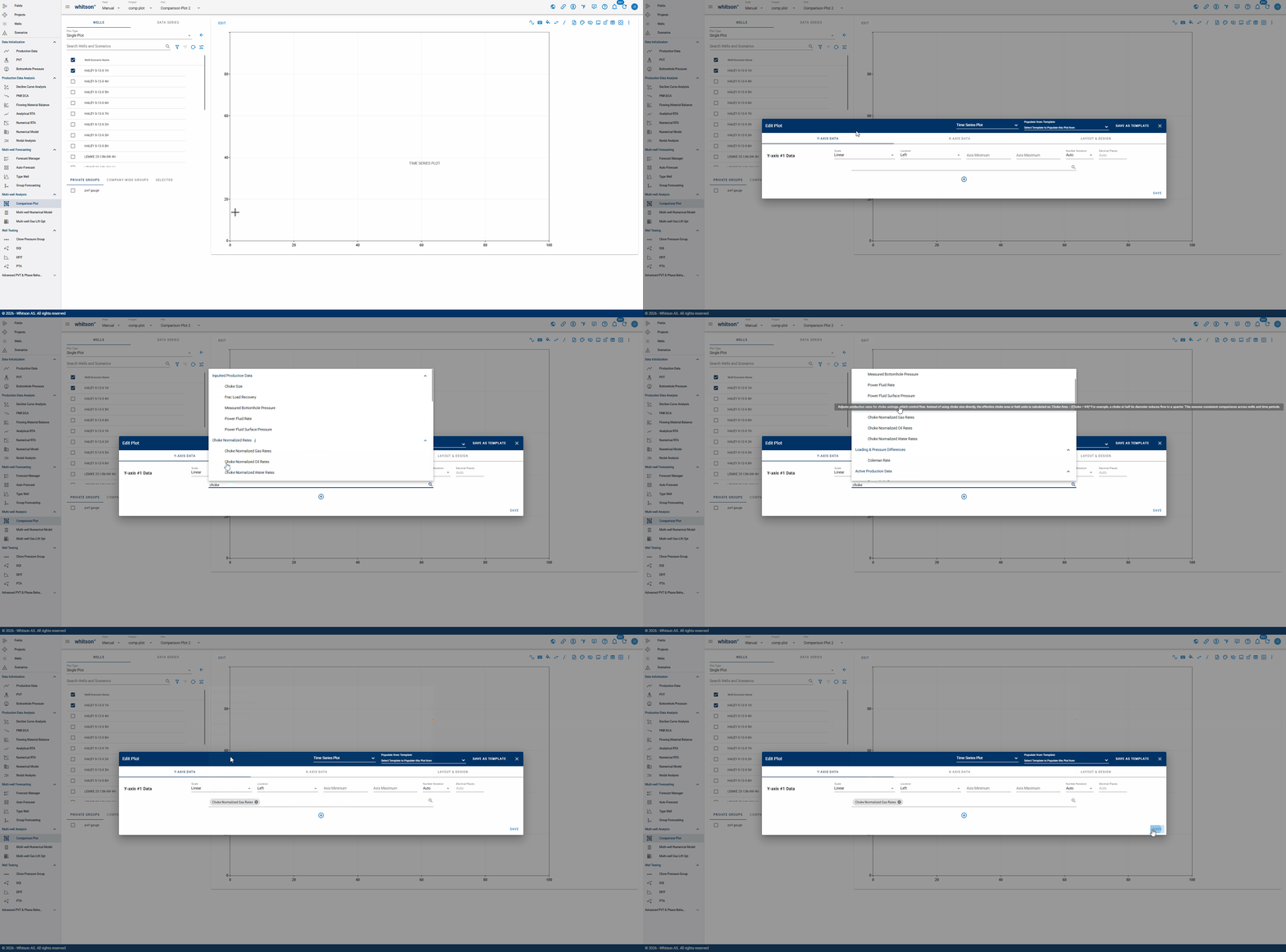
12.3. New Time Series: Choke-Normalized Rates
In well flowback analysis, choke-normalized rates are calculated to account for variations in choke settings, which affect the flow of oil and gas. A choke is the device that regulates the flow rate of produced fluids by limiting the well’s open area. To achieve meaningful comparisons, oil production rates are often normalized to reflect both lateral length (which correlates with productivity) and choke size (which controls flow).
Instead of dividing production by the choke size directly, a normalized choke-area factor is used to better capture the impact of the choke setting on flow rate. When the choke setting is expressed in 64ths of an inch, this dimensionless factor varies quadratically, rather than linearly, with choke diameter:
This equation converts the choke setting to a normalized area factor. For example, a choke set to half of its full-open diameter has one-quarter of the full-open area. Combining choke-area and lateral-length normalization provides a more accurate representation of production performance across wells and enables consistent time-series comparisons.
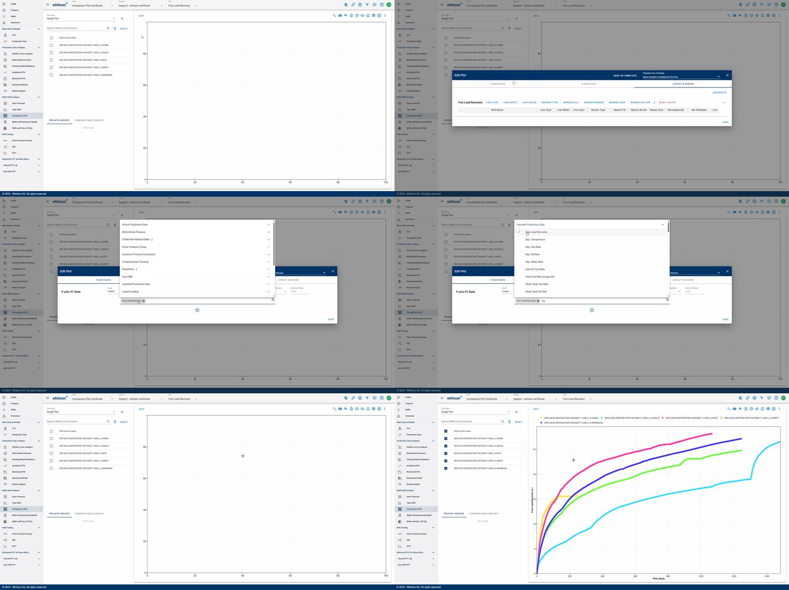
12.4. New Time Series: Frac Load Recovery
A crucial aspect of post-fracturing analysis is monitoring how much of the injected fluid is recovered during the flowback phase. This is typically tracked using the Cumulative Water per Fluid Pumped metric, which represents the total volume of water recovered relative to the amount initially injected.
Users can efficiently assess this recovery by utilizing the Frac Load Recovery variable. The Frac Load Recovery percentage is computed using the formula:
A higher Frac Load Recovery percentage suggests more extensive cleanup of the fracture network, whereas a lower percentage may indicate fluid retention within the formation and a potential impact on well performance.
12.5. Time Variables on the X-Axis
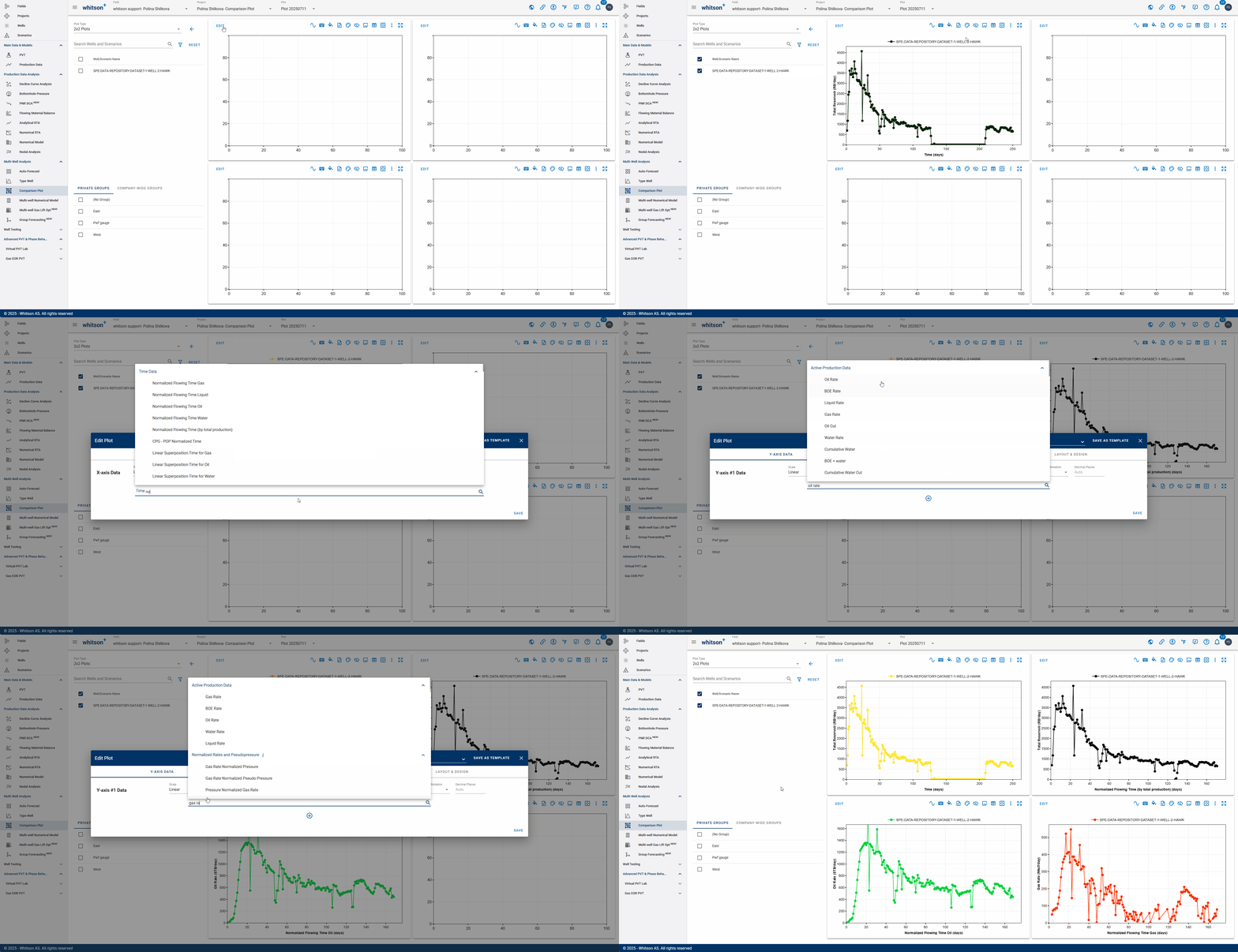
There are two main x-axis time options:
- Regular Time
- Normalized Flowing Time:
- Normalized Flowing Time by Stream: considers only time steps when the rate of the selected stream (oil, gas, or water) is nonzero, excluding periods with zero flow in that stream.
- Normalized Flowing Time by Total Production: considers a time step active when at least one production stream—oil, gas, or water—has a nonzero rate. It excludes only time steps when all three rates are zero.
- Normalized Flowing Time by Stream: considers only time steps when the rate of the selected stream (oil, gas, or water) is nonzero, excluding periods with zero flow in that stream.
12.6. PNR DCA Plots
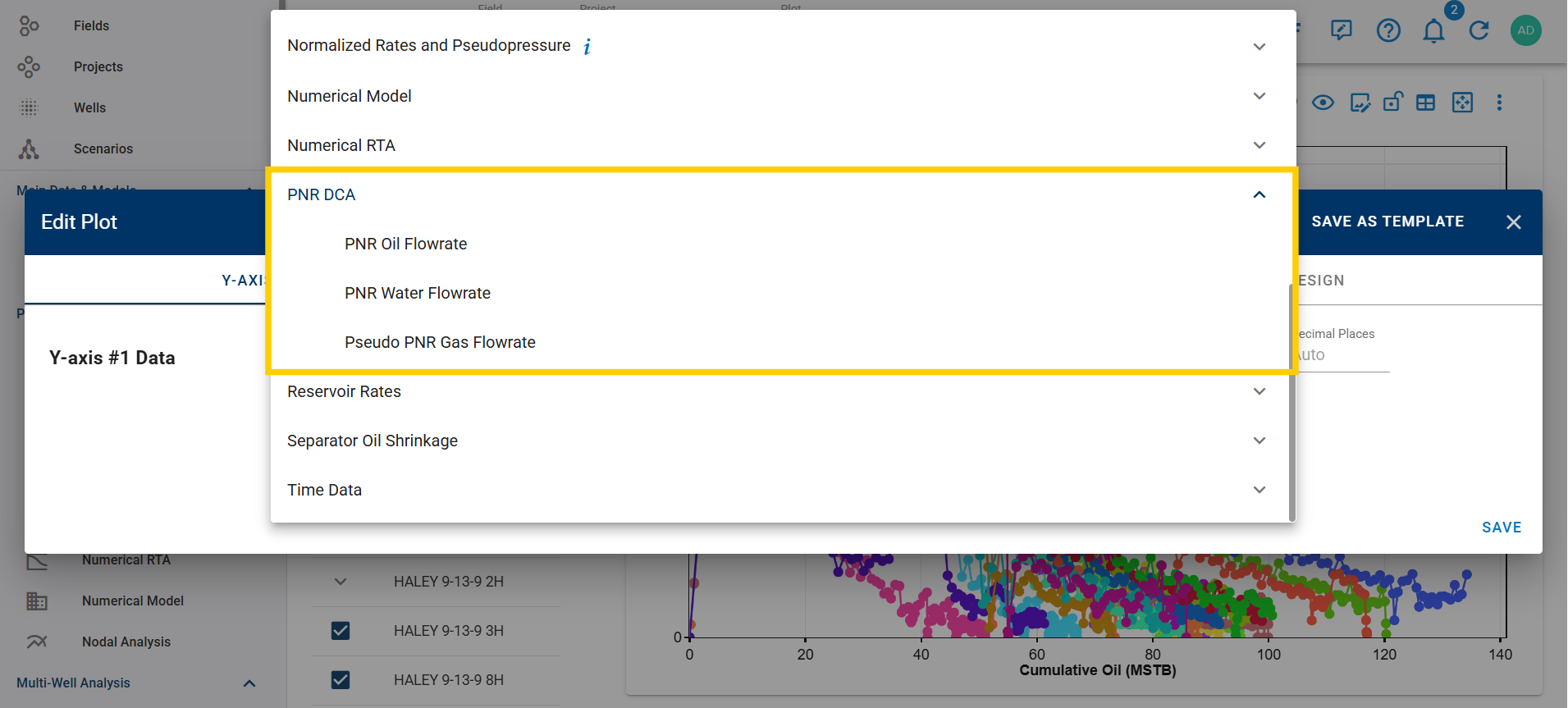
The Comparison Plot supports the visualization of decline curves based on pressure-normalized rates (PNR), enabling standardized comparisons of well performance across varying operating conditions. PNR DCA variables can be selected directly as axis data within the Comparison Plot.
12.7. Append DCA Forecast
Append well decline forecasts to your comparison plot to extend each history trace with a forecast trace for side-by-side benchmarking.
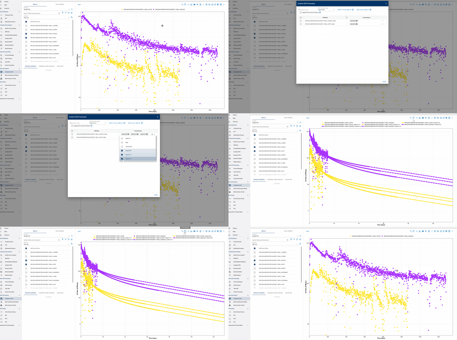
- Select the DCA Forecast button to view existing DCA forecasts in your project.
- Choose the wells for which you want to display the forecast.
- To apply the same forecast to all wells in your comparison plot, select it from the dropdown menu, then click Apply to All Wells.
- To apply a specific forecast to an individual well, select the forecast name you want to apply directly from the dropdown menu for that well.
- If a forecast is already selected, you can use the Add to All Wells button to append another forecast to all wells simultaneously.
- Choose how the forecast is aligned relative to production history:
- Append from End of History enabled: The forecast begins at the end of the historical data.
- Append from End of History disabled: The forecast begins at the first x-axis value displayed for the production history and overlaps the historical data.
-
Optionally, customize the forecast line and marker styles using the existing Layout and Design options.
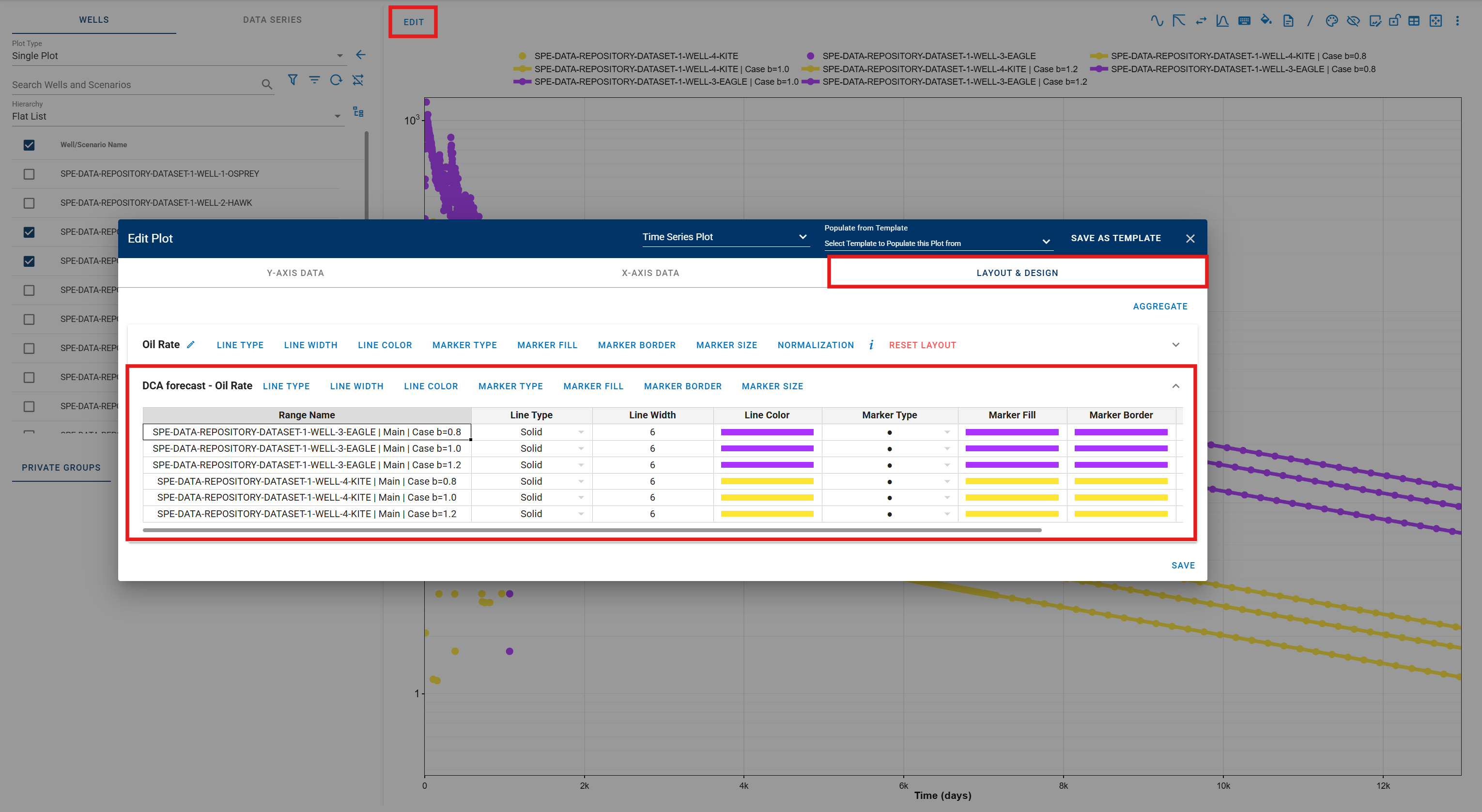
-
Click Save.
- All steps are shown above.
12.8. Append Typewell DCA Forecast
Append a typewell forecast built from a peer set to your comparison plot for quick benchmarking against a representative curve.
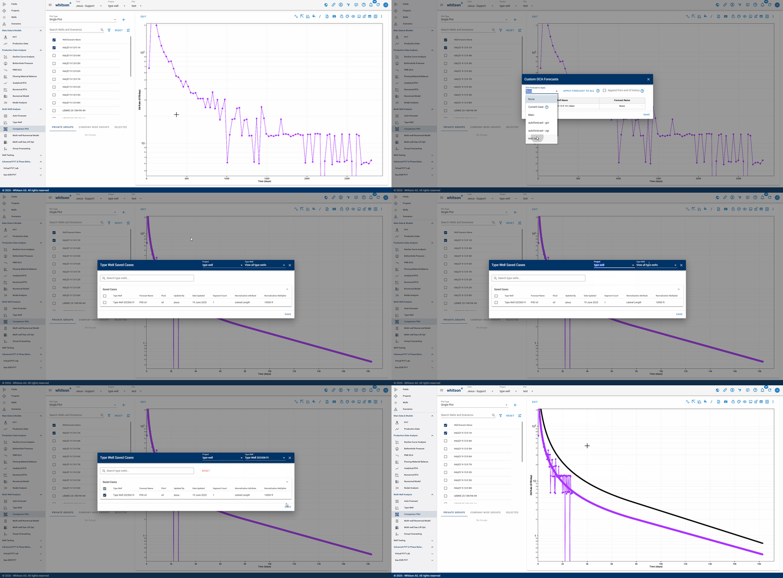
- Select the Typewell DCA Forecast button to view existing Typewell forecasts. Here, you can view forecasts from all projects within your field.
- Once you have chosen the project and type well, a summary of the saved cases will be available.
- Select the saved case you want to append to the comparison plot.
- Click Save.
- All steps are shown above.
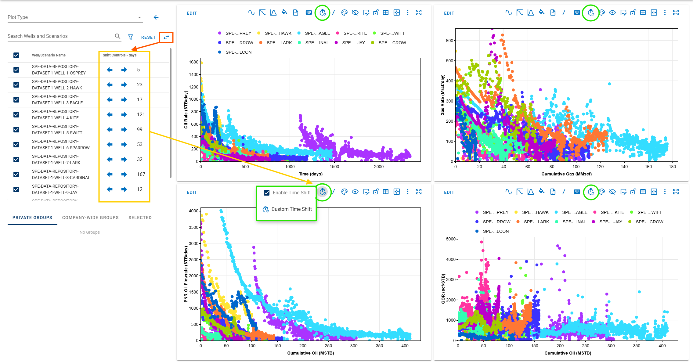
12.9. Time Shift
The time-shift feature allows users to align wells on plots by shifting selected wells along the time axis or adjusting their corresponding x-axis functions in time-series visualizations. Manual entry of shift values is also supported, which is useful for plots where the x-axis is not time-based (e.g., cumulative production).