Production Data - Separator Data
This page goes through the details of working with separator rates. Separator rates are typically available during flowback or if a single-well separator is installed.If you are working with stock tank rates, follow the information here instead Production Data - Stock Tank Rates.
Run PVT before running Common Process Conversion (Sep. Oil Shrinkage).
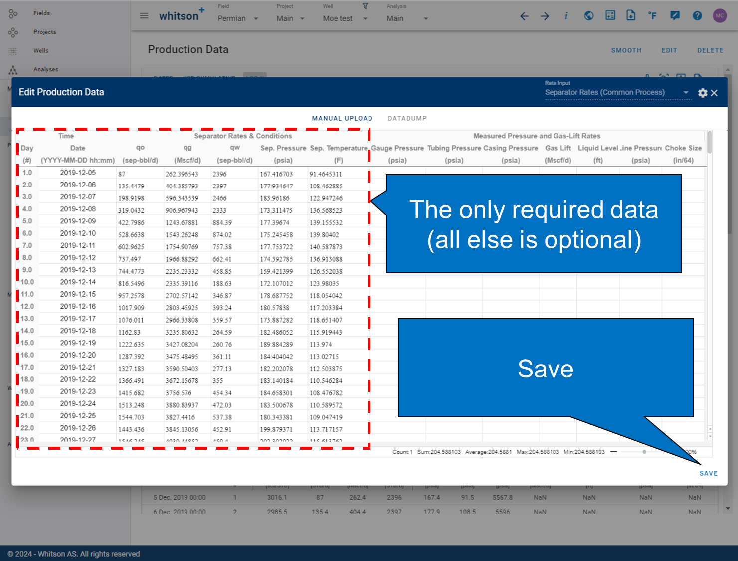
Required Data
-
Date: production data recording date
-
Separator Rates & Conditions
- qo: oil production rates at the separator (field: sep-bbl/d, SI/Metric: sep-m\(^3\)/d, SI/Metric Canada: sep-m\(^3\)/d)
- qg: gas production rates at the surface (field: Mscf/d, SI/Metric: 10\(^{-3}\)Sm\(^3\)/d, SI/Metric Canada: 10\(^{-3}\)Sm\(^3\)/d)
- qw: water production rates at the separator (field: sep-bbl/d, SI/Metric: sep-m\(^3\)/d, SI/Metric Canada: sep-m\(^3\)/d)
- Sep. Pressure: separator pressure (field: psia, SI/Metric: bara, SI/Metric Canada: kPaa)
- Sep. Temperature: separator temperature (field: F, SI/Metric: C, SI/Metric Canada: C)
-
Measure Pressure and Gas-Lift Rates
- Gauge Pressure: measured downhole gauge pressure (field: psia, SI/Metric: bara, SI/Metric Canada: kPaa)
- Tubing Pressure: tubing pressure (field: psia, SI/Metric: bara, SI/Metric Canada: kPaa)
- Casing Pressure: casing pressure (field: psia, SI/Metric: bara, SI/Metric Canada: kPaa)
- Gas Lift: gas lift injection rate if using gas lift (field: Mscf/d, SI/Metric: 10\(^{-3}\)Sm\(^3\)/d, SI/Metric Canada: 10\(^{-3}\)Sm\(^3\)/d)
- Liquid Level: measured depth of liquid level if using rod pump (field: ftMD, SI/Metric: mMD, SI/Metric Canada: mMD)
- Line Pressure: line pressure (field: psia, SI/Metric: bara, SI/Metric Canada: kPaa)
- Choke Size: choke size (field: 1/64 inch, SI/Metric: mm, SI/Metric Canada: mm)
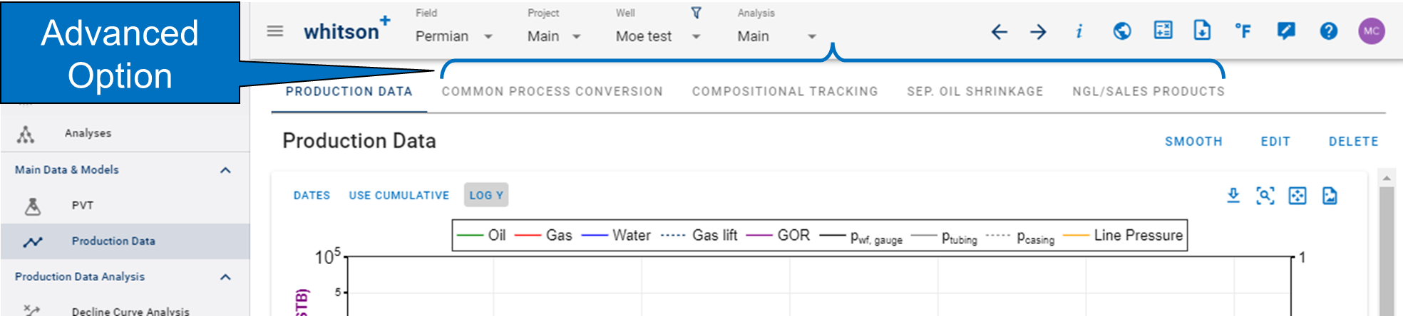
Separator Data Options
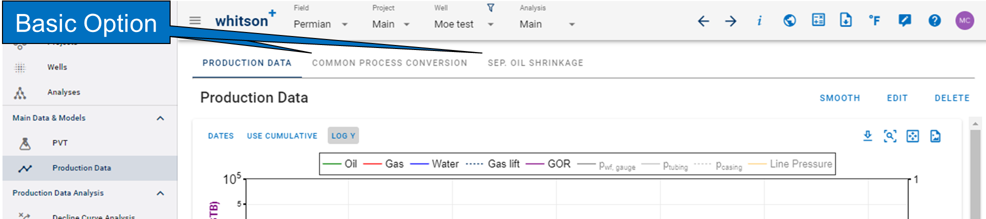
There is a basic (default option) and an advanced option. The advanced option can be turned as shown in the GIF below.
The picture below shows how Production Data looks like when the basic (default) option is run. The basic option calculates and databases the:
- common process rates
- daily separator oil shrinkage factors (SF) and flash factors (FF)
Additional values can be calculate if the Activate advanced compositional run is on, including
- daily wellstream compositions
- daily separator compositions
- daily stock tank compositions
- option to run daily NGL yield calculations
All of these are being run at the same time.
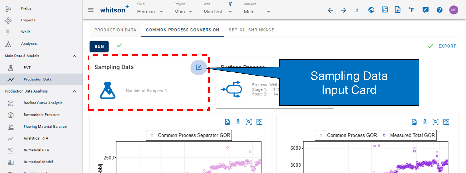
1. Sampling Data
The user will input any available sampling data for a given well. This data should be a representative sample, either; (1) reservoir representative, or (2) in-situ representative.
Note
Reservoir Representative: Any uncontaminated fluid sample produced from a reservoir is automatically representative of that reservoir.
In-situ Representative: A sample representative of the original fluid(s) in place.
At least one entry of sampling data is required before running any production data diagnostic modules (e.g. compositional tracking, separator oil shrinkage, and common process conversion). In the absence of sampling data, whitson+ utilizes the previouly inputted well fluid definition in fluid definition module.
Method
Each of the sample should come with the sampling date and one method by which the composition is defined. There are six available methods, namely:
- GOR
- API and GOR
- GOR and Saturation Pressure
- Dry Gas Composition
- Separator Compositions
- Fluid Composition
A more detailed description on each method, including the required input data, can be found here.
One has the option to upload sampling file(s) if they are available.
Once it has been inputted, the predicted wellstream composition can be seen. To delete a given sample, simply click the trash bin icon.
Mass Upload
For a more effective way to upload a large amounts of data sample, whitson+ provides solution with so-called mass upload feature. This is an option where user can easily upload any number of data sample in a quick.
Follow these steps:
- Download excel template provided by whitson+.
- Fill in all information on all samples. As of now, only two methods are possible for the use of this feature (e.g. API and GOR and Separator Compositions method).
- Upload the excel file to whitson+.
This feature requires that 'Advanced Compositional Run' is on.
The separator production data and fluid sampling data is used to predict daily:
- Wellstream Compositions
- Mole Rates
- Mass Rates
- Saturation Pressure and Type of Producing Wellstream
Wellstream Compositions
Compositions define the relative amounts of different components that make up a fluid. A wellstream composition represents the composition a well produces at one point in time. EOS models enable convenient and flexible calculations for describing phase behavior of petroleum fluids. However, to use an EOS model, a composition is needed in addition to pressure and temperature. Temperature and pressure are almost always available, but measured wellstream compositions every day are typically not. The purpose of this module is to make wellstream compositions readily available for every single well, every single day. The wellstream composition is calculated as given here.
Why do I need Wellstream Compositions over Time?
There are several reasons why engineers would like to know variations in wellstream compositions over time. Wellstream compositions can be used to, for example:
- Indicate when the well is: (i) producing at BHPs below the in-situ saturation pressure, (ii) producing from several layers with different in-situ fluid compositions, or (iii) experiencing gas coning in the perforated interval (most relevant for conventional reservoirs),
- Assist in history matching and production performance forecasting,
- compare well-to-well production behavior throughout a field in a consistent, “surface-process insensitive” manner – indicating differences in well performance and/or in-situ fluid spatal variations,
- Allocate oil and gas rates and/or components to individual wells,
- Assist in condensate tracking – study relative contributions from a condensate gas cap,
- Assist in fluid initialization and well classification exercises,
- Understand compositionally sensitive processes such as gas enhanced oil recovery,
- Study the sensitivity of surface process on rates, liquid yields and GORs,
- Perform separator train optimization,
- Normalize for changing separator conditions. Separator conditions might vary considerably over time, hence, part of the GOR variation seen over time is due to changing separator conditions. By knowing wellstream compositions over time one can express GOR in terms of a fixed surface process and remove “noise” in production data (“GOR normalization”),
- Assist in facility design.
Mole Rates
Molar rates, i.e. the total number of moles (\(n\)) produced every day, is calculated as, \(n = n_o + n_g = q_{om}/v_o + q_{gm}/v_g\), where \(q_{om}\) is the measured oil rate, \(v_{o}\) is the oil molar volume, the \(q_{gm}\) is the measured gas rate and \(v_{g}\) is the gas molar volume.
Gas rates, even when measured at sep. conditions, are reported at standard conditions, hence we can use the ideal gas law for the molar volume of the separator gas. The molar volume of the separator oil has to be calculated based on a EOS calculation.
Mass Rates
Mass rates, i.e. total mass (\(m\)) produced every day, is calculated as \(m = MW * n\), where \(n\) is the mole rate and \(MW\) is the average molecular weight of the wellstream.
Saturation Pressure & Type
If the wellstream composition changes over time, the saturation pressure of the producing wellstream will also change. The saturation pressure type (bubblepoint or dewpoint) might also change depending on fluid system. For a specific wellstream composition and reservoir temperature, the producing fluid composition is calculated every day.
Want to know more? Here is a presentation on compositional tracking.
3. Separator Oil Shrinkage & Flash Factor
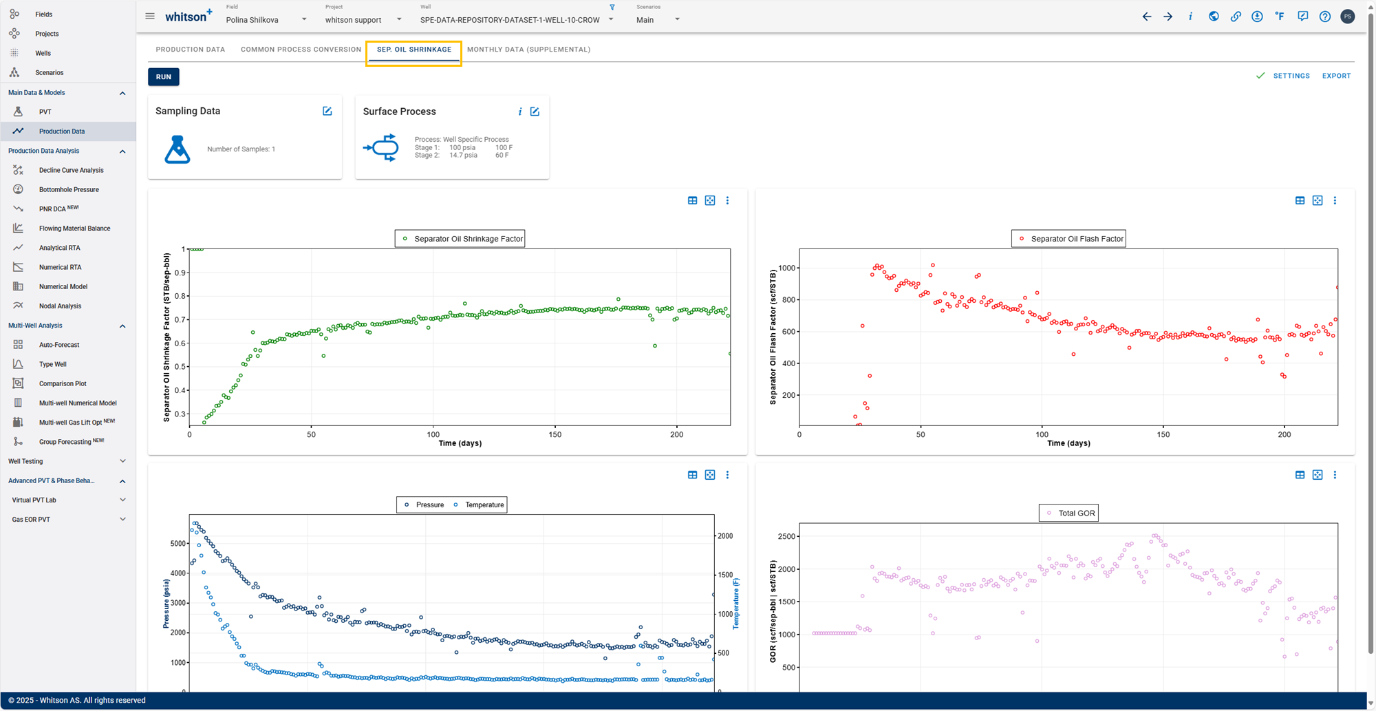
The separator production data and daily wellstream compositions are used to calculate daily
- Separator Oil Shrinkage Factors
- Separator Oil Flash Factor
- Total Producing GOR
Separator Oil Shrinkage Factor
Separator-oil shrinkage factor, or just shrinkage factor (SF), is the fraction of metered separator oil rate that remains (transforms into) stock-tank oil after further processing down to standard conditions of 1 atm and 60 °F (Hoda & Whitson 2013). In layman's terms, the shrinkage factor quantifies the decrease in oil volume from separator conditions to stock tank, and the magnitude can range from < 0.65 - 0.99.
Flash Factor
Separator-oil flash factor, or just flash factor (FF), is the ratio of liberated gas from metered separator oil after further processing down to standard conditions of 1 atm and 60 °F. In Layman’s terms, the flash factor accounts for the increase in gas volume from separator conditions to stock tank. It is the exact reason why oil is shrinking, i.e. gas is coming out of solution. The magnitude of the flash factor can range from 5 - 1000 scf/STB (and even more).
Total GOR
Total producing GOR (\(R_p\)) can be calculated easily when knowing shrinkage factor and flash factor: \(R_p = R_{p,sep}/SF + FF\). A shrinkage factor is always associated with a flash factor and is literally the solution GOR of the separator oil (\(R_{s,sep}\)).
Requirements to Estimate Wellstream Compositions:
- A properly tuned EOS model
- An estimate of a wellstream comp – “seed feed”
- Separator volumetric rates (GOR)
- Separator conditions (Tsep, psep)
Requirements to Calculate Shrinkage Factor and Flash Factor Daily:
- Consistent fluid description
- Fundamental physical and thermodynamic principles
Want to know more? [Here is a presentation on separator oil shrinkage and flash factors.](\files\technical-presentations\sep-shrinkage.pdf
4. Common Process Conversion - Convert Rates to a Common Surface Process
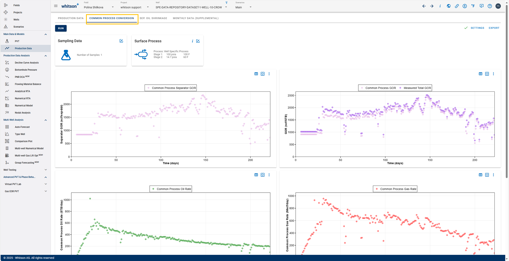
The separator production data and daily wellstream compositions are used to calculate daily:
- Common process separator GOR
- Common process GOR
- Common process rates
The common process rates are the rates that should be used when modeling the wells history.
Note
Common Process referes to rates and GORs that are re-processed through a fixed separator process.
Common Process Conversion - What is It?
Black oil tables are generated assuming a fixed surface process, but in reality, separator conditions change through time. Hence, there is a risk for inconsistencies between the rates used in history matching (assumes constant separator conditions) and the actual measured rates (changing separator conditions in the field). If surface process separator conditions are changing significantly over time, a “correction” to a set of constant separator conditions might be needed for:
- Consistent well-to-well performance comparison
- Consistent usage of black oil tables in history matching (using RTA/PTA or res. simulation)
- Consistent analysis of CGR performance over time
The correction is referred to as a common process conversion, as we “convert” the rates processed through changing separator conditions to a "common process".
Want to know more? Here is a presentation on common process conversion.
What is the difference between shrunk rates and common process rates?
First, both of these represent a conversion of rates from separator conditions to stock tank conditions.
Shrunk Rates
Here, we take the actual separator conditions at every point in time (separator pressure and temperature) and use them to calculate what the oil and gas volumes would be at stock tank conditions.
Best for: matching real production / sales numbers.
Common Process Rates
Here, the changing separator conditions are only used to determine what the fluid coming from the well looks like (the flowing wellstream).
After that, we ignore the changing surface setup and always process the fluids through one fixed separator process, the same one used to generate the PVT and black oil tables.
That is why we call it the "common process".
So, the rates are always calculated using a consistent surface setup.
Best for: engineering workflows and simulation, as it ensures consistency with PVT data.
In Its Simplest Form
-
Shrunk Rates:
“Use the separator conditions from that day, for actual sales / allocation.” -
Common Process Rates:
“Pretend the plant conditions were always the same, for engineering consistency.”
5. Sales Products
This feature requires that 'Advanced Compositional Run' is on.
5.1. Definition
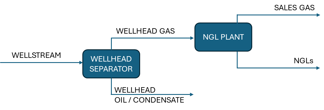
Wellhead Gas
- The gas coming out of the separator at the wellhead and entering the NGL plant.
- This is the actual gas stream processed for NGL extraction.
Sales Gas
- The final gas product after the NGL plant.
- Stripped of heavier hydrocarbons (NGLs), making it drier and pipeline-ready, i.e. sales gas.
Fat Gas (a.k.a. Wet Gas)
An artificially reported stream in some production databases. It basically recombines:
- Gas coming out of the separator (Wellhead Gas)
- Condensate from the separator (converted to gas-equivalent)
Important: this stream does not exists as a real gas stream but is mostly used for reporting, to track total hydrocarbon content as a single gas stream.
5.2. Natural Gas Liquids (NGL)
In this module, daily NGL rate (\(q_{NGL}\)) and NGL yield are predicted. The required input for the user is NGL efficiencies (\(e\)).
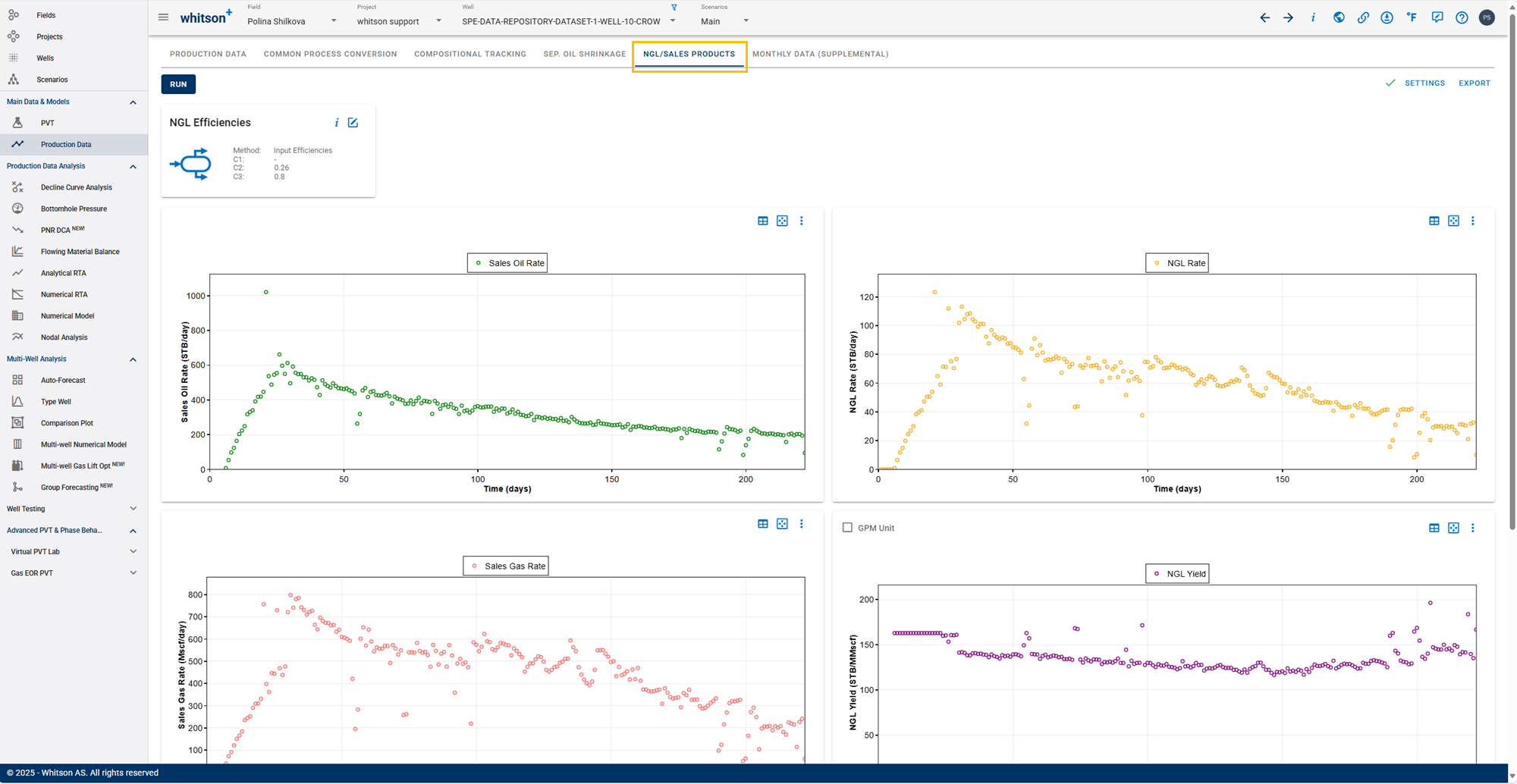
5.2.1. Recovery Method
The process of removing NGL's is acknowledged as NGL recovery. There are four methods to calculate NGL recovery available in whitson+:
- Dewpoint Control: controls hydrocarbon and water dew points of natural gas through mechanical refrigeration.
- Cascade Refrigeration: uses two refrigeration ciscuits thermally connected by a cascade condenser.
- Gas Sub-cooled Process (GSP) Deep Recovery: develops a source of reflux to increase \(C_2\) recovery with the conventional design.
- Input Efficiencies
Each method has a list of components according to the EOS model used. The default efficiencies for each method is given in Table 1. Using one of this default values is good for the starting point of the NGL efficiency, the values can be changed as desired.
| Component | Dewpoint Control | Cascade Refrigeration | GSP Deep Recovery | Input Efficiencies |
|---|---|---|---|---|
| \(N_2\) | 0 | 0 | 0 | 0 |
| \(CO_2\) | 0 | 1 | 1 | 0 |
| \(H_2S\) | 1 | 1 | 1 | 0 |
| \(C_1\) | 0 | 0 | 0 | 0 |
| \(C_2\) | 0.25 | 0.65 | 0.95 | 0.5 |
| \(C_3\) | 0.80 | 0.97 | 0.99 | 1 |
| \(C_4+\) | 0.97 | 1 | 1 | 1 |
5.2.2. Calculations
To predict the NGL yield and NGL rate correctly, the following inputs are fundamental:
- daily measured oil and gas rates (\(q_o\) and \(q_g\))
- daily gas moles (\(n_{gas}\))
- daily composition of surface gas (\(y_i\))
- NGL efficiencies (\(e\))
Gas and oil production rates are used to calculate \(n_{gas}\) and (\(y_i\)). In whitson+, \(n_{gas}\) and (\(y_i\)) are calculated in compositional tracking module.
Mole of NGL sales is written as:
Liquid phase mole fraction of each component can be defined
NGL molecular weight and specific gravity are expressed as follows
Finally, the NGL rates and thus NGL yield can be solved for each production day
The units of NGL rate is STB/d and NGL yield is STB/MMscf (or gallon per 1,000 cubic feet, GPM).
5.2.3. Ethane Rejection vs. Ethane Recovery
When demand for ethane, and therefore ethane prices, are low relative to dry natural gas prices, natural gas processing plant operators may choose to leave ethane in the processed natural gas (provided the processed natural gas meets pipeline specifications) and sell it into the natural gas market at its heat value. This process is known as ethane rejection.
When ethane prices rise higher than natural gas prices on a heat-value equivalent basis, natural gas processing plant operators may choose to recover the ethane along with other NGPLs and sell it at their market value into the petrochemical sector. This process is known as ethane recovery.
Most recovery units are built for both ethane recovery and ethane rejection, and when operated in ethane rejection mode the ethane recovery (NGL efficiency) is low (e.g. 40%), while when operated in ethane recovery mode the ethane recovery (NGL efficiency) is high (e.g. 90%)
6. Example: Working with Separator Data
Separator data can be tricky to work with, so in this section we'll focus on how you can efficiently work with and handle separator rates in whitson+. Learn the most important things in less than 30 minutes.
Info
The examples shown in the videos below use the "Default EOS option" in whitson+ (more info here). Hence, if you are using a custom EOS, your results will be slighly different for the rest of these examples. However, the main objective of this is to learn the practicalities of the software, so it's not important in this context.
6.1 Fluid Definition with Separator Data
- In the Wells module, click ADD WELL up to the right.
- Add well with name for example: Separator Data Example.
- Click SAVE.
- Download the relevant data here.
- Go to the PVT module in the navigation panel.
- Open the Reservoir Fluid Composition Input Card.
- Change the Method from "GOR" to "Separator Compositions".
- Copy the right data from The Excel Sheet and paste it into the relevant cells.
- Click HOFFMAN QC:
- NB:The blue dots overlay the grey line, indicating the separator oil and gas compositions are in equilibrium. Occasionally, there may be significant differences in Nitrogen due to its small quantities, but it can be ignored. The most important is that the majority of C1 to C6 is on the line, also the C7+ is decent.
- Read more about HOFFMAN QC here.
- Click SAVE.
- Check the predicted fluid composition by clicking the "eye icon".
- Check the black oil table.
- All steps are shown in the .gif above.
6.2 Upload Production Data: Rates Measured at Separator Conditions
- Download the relevant data here.
- Go to the Production Data module.
- Click UPLOAD up to the right.
- Select the DATADUMP.
- Drop the data file into the DATADUMP box in the front end.
- Click SAVE.
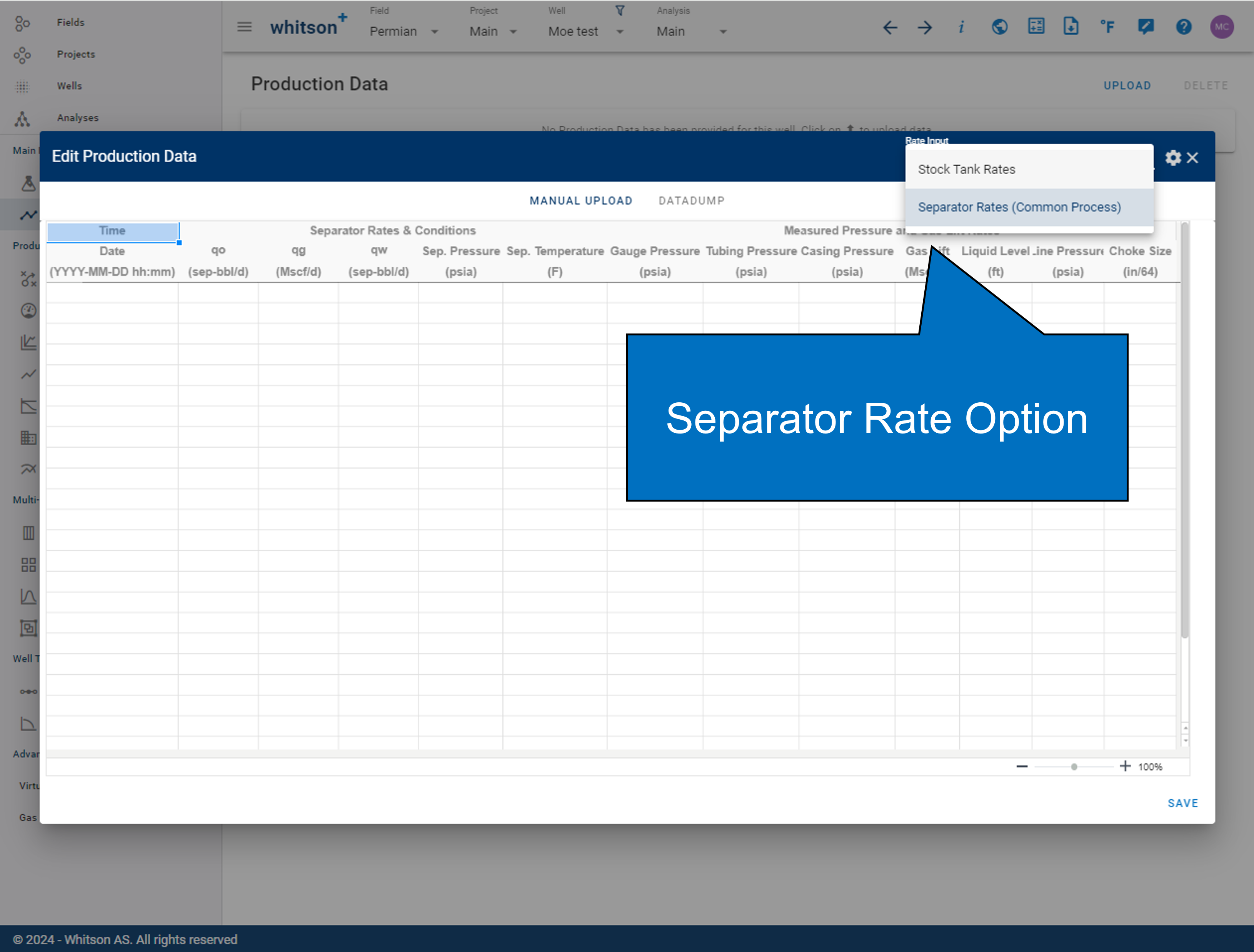
- Click EDIT.
- Change the Rate Input from Stock Tank Rates into Separator Rates (Common Process).
- Click SAVE.
- You’ll get the prompt "Calculation of Common Process Rates will be launched".
- Click YES.
- All steps are shown in the .gif above.
6.3 Common Process Conversion
- In the Production Data module.
- Click on the Common Process Conversion tab.
- The calculation is automatically done upon uploading the separator rates, but you can re-run if some changes have been made and are not reflected in the common process rate.
- All steps are shown in the .gif above.
- Read more about Common Process Conversion here.
6.4 Separator Oil Shrinkage Calculations
- In the Production Data module.
- Click on the Sep. OIL SHRINKAGE tab.
- The calculation is automatically done upon uploading the separator rates, but you can rerun if some changes have been made and are not reflected in the common process rate.
- Check Separator Oil Shrinkage Calculations.
- All steps are shown in the .gif above.
- Read more about Separator Oil Shrinkage here.
6.5 Sales Products - NGL Yield vs Time
- In the Production Data module.
- Click the NGL/SALES PRODUCTS tab up to the right.
- Open the NGL Efficiencies input card.
- Change the NGL Recovery Method to the Dewpoint Control.
- Click SAVE.
- Click RUN.
- All steps are shown in the .gif above.
- Read more about Sales Products - NGL calculation here.
6.6 Numerical RTA
In the Numerical RTA module.
- First RUN: Default values.
- Click RUN.
- This run will give us the initial simulation with the default input values.
- Second RUN: we can proceed to adjust the values as per the data provided in the Excel sheet here:
- Provide the relevant Fluid Initialization data.
- Provide the relevant Well data.
- Open the Relative Permeability input card, provide the relevant Relative Permeability data and click save.
- Click RUN, this second run should give you a much better match of the GORs and water cuts (you may adjust the relative permeabilities further if you want).
- All steps are shown in the .gif above.
Info
You will only need to re-run (click RUN) the numerical RTA module when you update any of the following parameters: PVT, Swi, Fcd, relative permeability, pressure-dependent permeability (gamma matrix/fracture) or initial pressure.
6.7 Numerical Model
- To transfer the results from the Numerical RTA module into the numerical model, click EXPORT at the top of the Interpretation menu in the Numerical RTA module.
- Read the pop-up box text and click YES. This exports the results into the Numerical Model.
- In the numerical model, click RUN
- All steps are shown in the .gif above.
References
[1] Carlsen M., Dahouk, M., Mydland, S. and Whitson C., Compositional Tracking: Predicting Wellstream Compositions in Tight Unconventionals, IPTC-19596-MS, Society of Petroleum Engineers, 2020.
[9] U.S. Energy Information Administration 2021, accessed November 18, 2021.