Numerical RTA - Technical Description
1. Theory
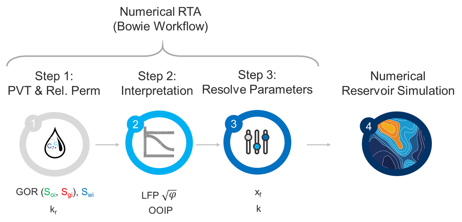
The numerical RTA module is designed based on the workflow proposed by Bowie and Ewert (2020) in URTeC 2967. A webinar about the workflow is available here.
1.1. What are the inputs and outputs to Numerical RTA?
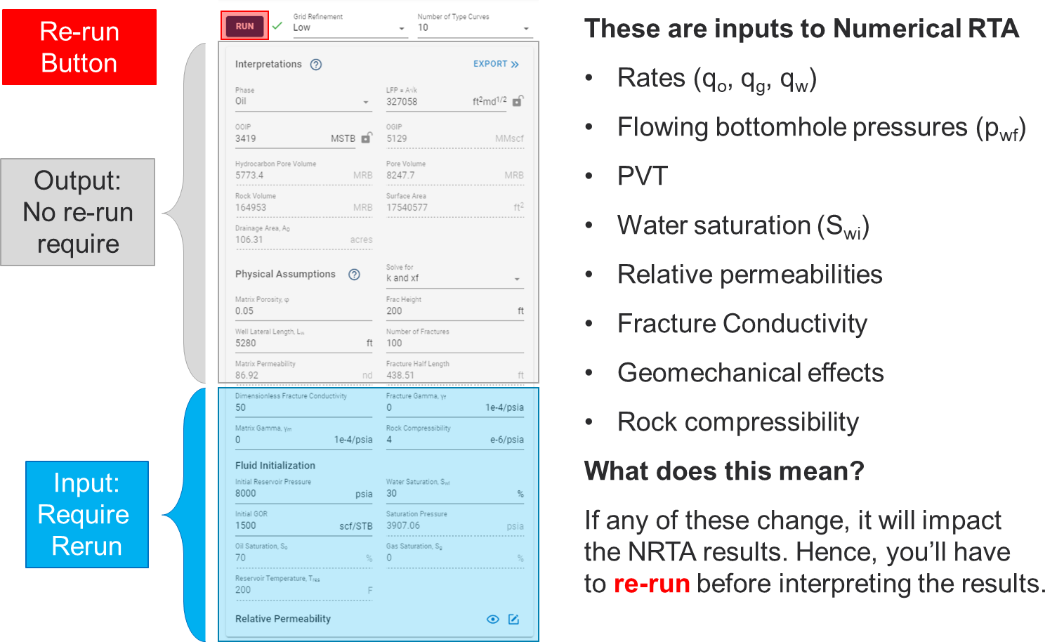
When will we have to re-run numerical RTA?
If you change any of the items above in grey (e.g. LFP, OOIP, OGIP \(\phi\), \(x_f\), \(k\), \(L_w\), \(h\) and \(N_f\)), you do not have to re-run the numerical RTA feature.
1.2. Numerical RTA - Practical Aspects
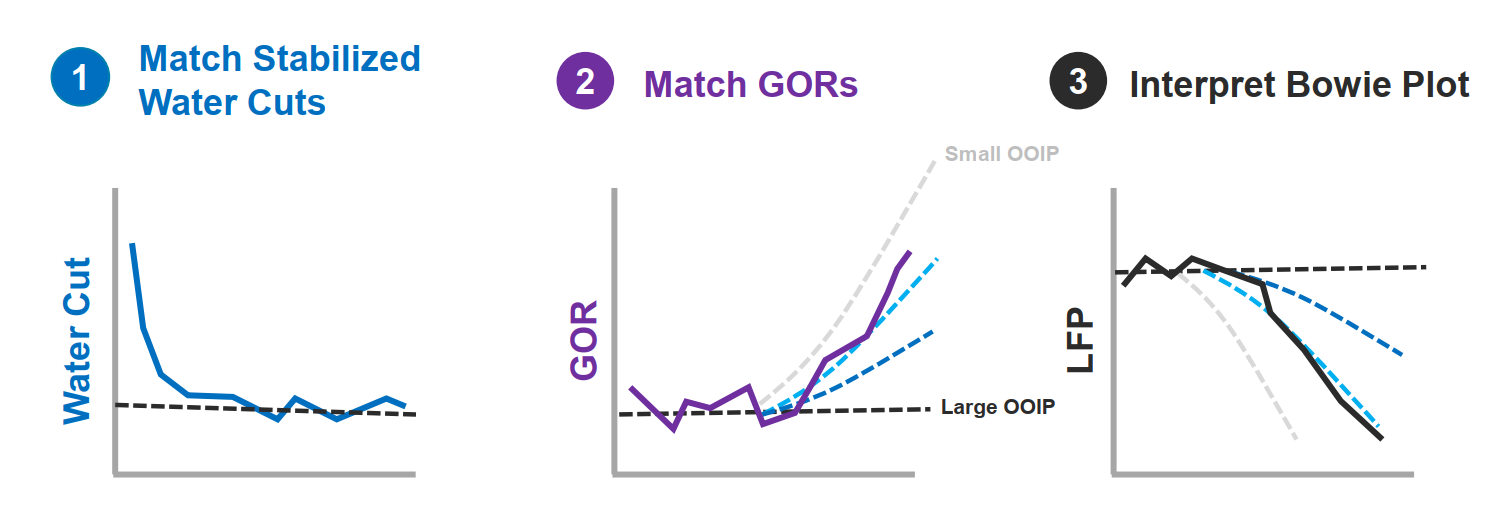
Before you interpret the "Bowie plot" ensure that you match stabilized water cuts and producing GORs.
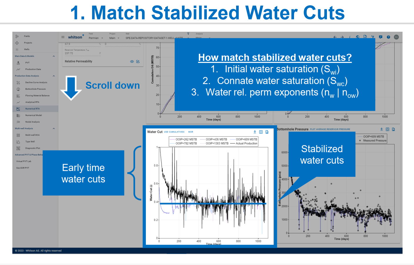
Matching water cut can primarily be achieved by changing either of these parameters, i.e. initial water saturation, connate water saturation and relative permeability exponents.
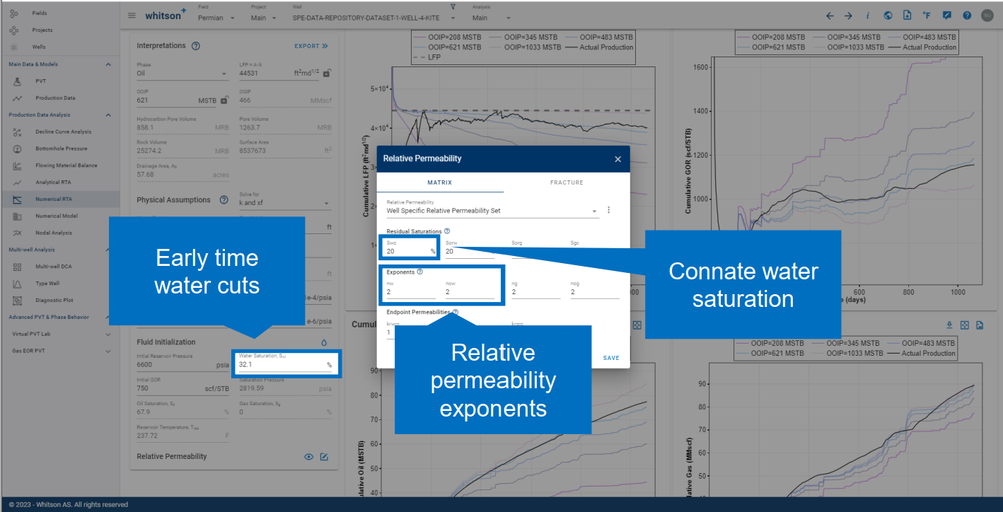
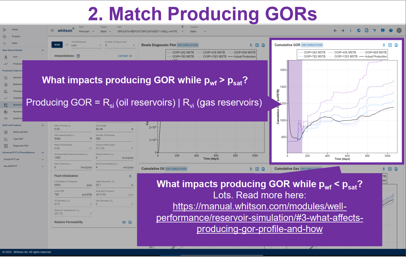
Producing GOR is a function of many parameters, including PVT, relative permeabilities, fracture conductivity, pressure dependent permeability and flow regime. Read more -->here<--.
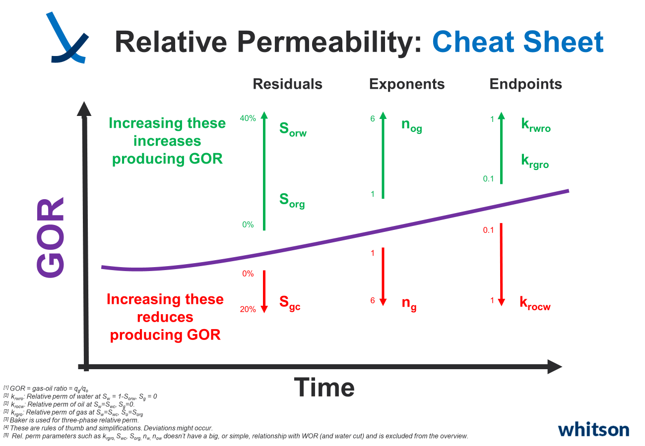
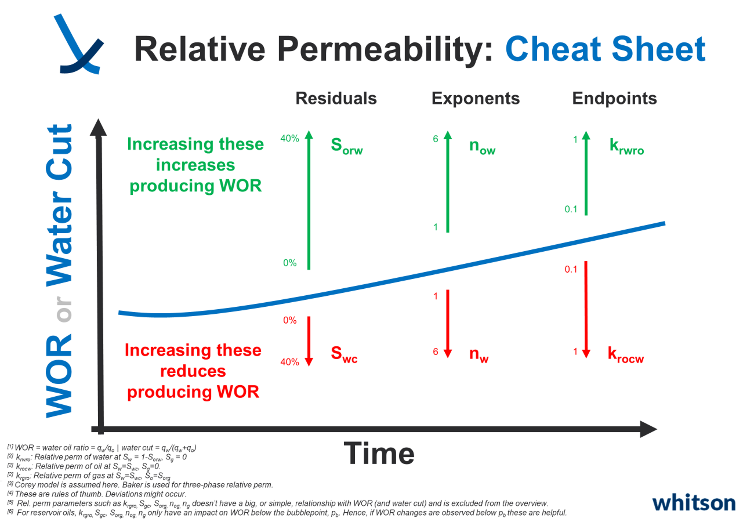
1.3. Relative Permeability Cheat Sheets
Understanding how relative permeabilities affect Gas-Oil Ratio (GOR) and Water-Oil Ratio (WOR), or water cut, can be tricky. It often takes experience, with engineers having their preferred parameters to tweak for achieving specific changes in simulated GOR, WOR, or other ratios. To simplify this, especially for beginners, we've created cheat sheets to help out.
GOR and \(S_{org}\)
To understand the relationship between GOR and \(S_{org}\), it is necessary to take a look at the equation for producing GOR:
Just to simplify things slightly, it can assume that \(r_s\) is 0
The producing GOR is a combination of PVT properties and relative mobilities (\(k_{rg}\)/\(k_{ro}\)).
Reducing the \(S_{org}\), will reduce \(k_{rg}\)/\(k_{ro}\) (example below), and hence reduce producing GOR.
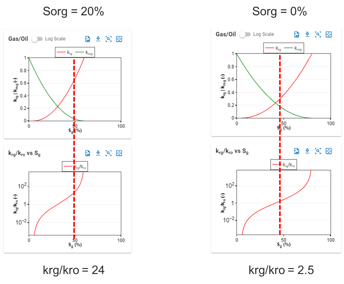
However, the relative reduction in \(k_{rg}\)/\(k_{ro}\) (and hence relative GOR reduction) will be a function of what the \(S_g\) is.
\(S_g\) is a function of fluid type (i.e. less gas comes out of solution of a low GOR oil with \(R_{si}\) = 500 scf/STB vs a near-critical fluid with \(R_{si}\) = 3500 scf/STB).
For the example below:
- If e.g. \(S_g\) is 50% (i.e. a more gassy fluid), the difference by changing \(S_{org}\) down to 0% would mean a reduction in \(k_{rg}\)/\(k_{ro}\) from 24 down to 2.5 (example). Order of magnitude difference.
- If e.g. \(S_g\) is 10% (i.e. a less gassy fluid), the difference by changing \(S_{org}\) down to 0% would mean a reduction in \(k_{rg}\)/\(k_{ro}\) from 0.01xx to 0.01yy (example). Almost no difference.
1.4. Underlying Assumptions - 1D Reservoir Model
All the simulations in this module are performed with a so-called "symmetry element" model, in which the numerical model is one-quarter of a fracture, as highlighted by a red-lined box in Fig. 1. In addition, this module assumes a so-called 1D numerical model, i.e. no flow contribution beyond the frac-tips (\(x_f\) = \(x_e\)) or height beyond the frac height (\(h_f\) = \(h\)). Note that there is only one zone permeability (i.e. no enhanced fracture region with a different permeability). Infinite conductive fractures are assumed.
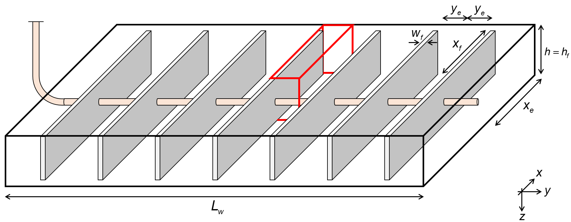
Fig. 1: Wellbox model
1.5. Three Fundamental Relationships
To understand the numerically assisted RTA workflow, the following two parameters are defined, i.e. a modified linear flow parameter (LFP') and original oil in place (OOIP):
in which \(\phi\) is porosity, \(A\) is area, \(k\) is permeability, \(N_f\) is number of fractures, \(h_f\) is the fracture height, \(x_f\) is the fracture half length, \(S_{wi}\) is the initial water saturation and \(B_{ti}\) is the total formation volume factor.
Total Formation Volume Factor
The original (surface) oil in place (OOIP) is generalized to represent both reservoir oil and reservoir gas condensate systems, using a consistent initial total formation volume factor definition (\(B_{t}\) ). Read more here.
For a given (i) well geometry (1D model described above), (ii) fluid initialization (PVT and initial water saturation), (iii) relative permeability relations, and (iv) bottomhole pressure (BHP) time variation (above and below saturation pressure), three fundamental relationships exist in terms of LFPꞌ and OOIP. These relationships provides the foundation for numerical RTA.
For any two wells:
| Condition | Implication |
|---|---|
| Same value of LFP' | rate performance will be identical for the two wells during infinite-acting (IA) period |
| Same ratio LFPꞌ/OOIP | GOR and water cut behavior will be identical for the two wells at all times, IA, transitional and boundary dominated (BD) |
| Same values of LFPꞌ and OOIP | rate performance will be identical for the two wells at all times, IA and BD. |
These observations lead to an efficient, semi-automated process to perform rigorous RTA, assisted by a symmetry element numerical model.
To remind ourselves that these relationships hold for the 1D model presented above a few different examples are provided below.
1.5.1. Same LFP', same IA performance
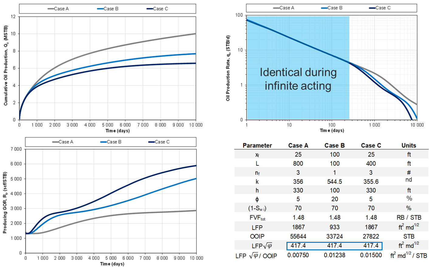
Fig. 2a: Same LFP', different OOIP
1.5.2. Same LFP'/OOIP ratio, same GOR
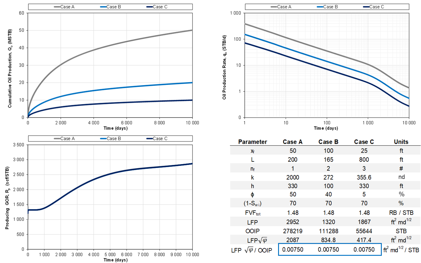
Fig. 2b: Same LFP'/OOIP ratio
1.5.3. Same LFP' and OOIP, same performance
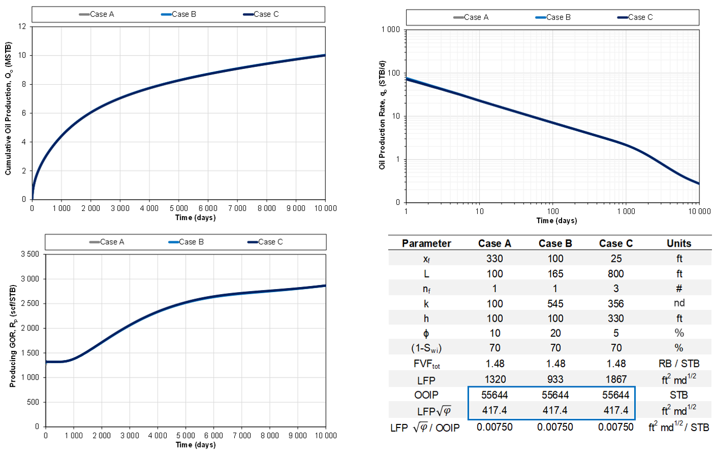
Fig. 2c: Same LFP' and OOIP
1.6. Computing Original Gas in Place with Adsorption
Shale reservoirs possess a remarkable capacity to store methane through a process known as "adsorption." This involves gas molecules adhering to the organic material within the shale, creating a near-liquid state of condensed gas. A useful analogy is to envision a magnet sticking to a metal surface or lint clinging to a sweater, illustrating the concept of adsorption versus absorption, where one substance is trapped inside another like a sponge soaking up water. The adsorption process is reversible due to its reliance on weak attraction forces.
Compared to conventional reservoirs, shale reservoirs can store significantly more gas in the adsorbed state, even when compression is applied at pressures below 1000 psia. Notably, the gas stored in shale is predominantly held in the adsorbed state, as opposed to being free gas. This is because the volume of the cleat or fracture system within shale is relatively small compared to the overall reservoir volume. As a result, the pressure volume relationship is commonly described through the desorption isotherm alone.
Langmuir Isotherm
The release of adsorbed gas is commonly described by a pressure relationship called the Langmuir isotherm. The Langmuir adsorption isotherm assumes that the gas attaches to the surface of the shale, and covers the surface as a single layer of gas (a monolayer). At low pressures, this dense state allows greater volumes to be stored by sorption than is possible by compression.
The typical formulation of the Langmuir isotherm is:
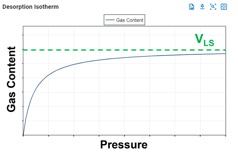
Langmuir Volume, VLS
The Langmuir volume is the maximum amount of gas that can be adsorbed by a shale at an "infinite pressure". The plot below of a Langmuir isotherm demonstrates that gas content asymptotically approaches the Langmuir volume as pressure increases to infinity.
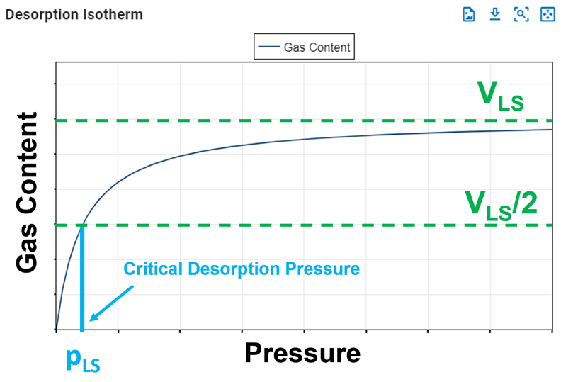
Langmuir Pressure, pLS
The Langmuir pressure, or critical desorption pressure, is the pressure at which one half of the Langmuir volume can be adsorbed. As seen in the figure below, it changes the curvature of the line and thus affects the shape of the isotherm.
Computing Original Gas in Place (OGIP)
Ambrose et al.[1] argue that the free OGIP must be corrected for the adsorbed gas that occupies some of the hydrocarbon pore volume (HCPV). If porosity is estimated from core plugs where core preparation has removed the adsorbed gas, then the OGIP will be overestimated.
The convention of reporting OGIP when adsorption is included, is to report it in units of scf/ton (standard cubic feet per short ton). For a fluid system having only dry/wet gas and water, the total OGIP is
where
and with \(C_1\approx 5.7060\) and \(C_2\approx1.318\cdot10^{-6}\) are unit conversion factors. The shale saturation is capped at \(1-S_{wi}\), meaning the maximum amount of shale you can have is the entire HCPV. Hence, this will make the results independent of the adsorption numbers when violating this constraint.
The OGIP resolved in the ARTA and GFMB features yields the free OGIP. We can use this volume to compute the rock mass, which in turn can be used to calculate the adsorbed OGIP. Multiplying equation \eqref{eq:freegasperton} with the rock mass (\(G=\hat{G}_f m_r\)) gives the free OGIP in units of scf. Solving for the rock mass yields
This rock mass can then be multiplied by equation \eqref{eq:adsorbedgasperton} to get the adsorbed OGIP in scf, i.e.,
Total Compressibility when Adsorption is ON
In order to honor mass balance, it becomes necessary to modify total system compressibility when accounting for adsorption. Total system compressibility can be determined using the following equation:
The derivation of this equation is shown here and is constructed upon Ambrose et al.[1].
2. Numerically Assisted RTA Workflow
The fundamental relationships outlined above represent the basis of the suggested workflow. The suggested workflow, can be divided into 8 steps, all of which are automated in the workflow through whitson+.
Numerical RTA workflow
- Create a numerical model, the "template model", that is large enough to behave infinite acting (=large OOIP) for the entirety for the historical time. In practice, this means to create a single fracture, numerical model with a large distance to the closest boundary. Assign a relevant fluid initialization (PVT and \(\mathrm{S_{wi}}\) and relative permeability relations. More details about the "template model" used in whitson+ can be found here.
- Run this “infinite acting model” controlled with the wells actual measured bottomhole pressure (\(\mathrm{p_{wf}}\)).
- Calculate the ratio between the actual measured oil rates and infinite acting model oil rates: r = \(\mathrm{q_{o,actual}}\)/\(\mathrm{q_{o,IA}}\). Alternatively, one can use the cumulatives to reduce noise: r = \(\mathrm{Q_{o,actual}}\)/\(\mathrm{Q_{o,IA}}\).
- Calculate the daily “LFP'” by multiplying the daily ratio r (Step 3) with the known LFP' of the infinite acting, single fracture model (Step 1). (a) a horizontal flat line indicates infinite acting, linear flow (b) deviation below this line represents transitional flow or boundary dominated flow, (c) the magnitude of the flat line indicates the LFP'.
- Repeat Step 1-2 for multiple, smaller OOIP volumes (reduce distance to closest boundary in the "template model", as outlined here). This results in several “type curves” with each its own LFP'/OOIP ratio.
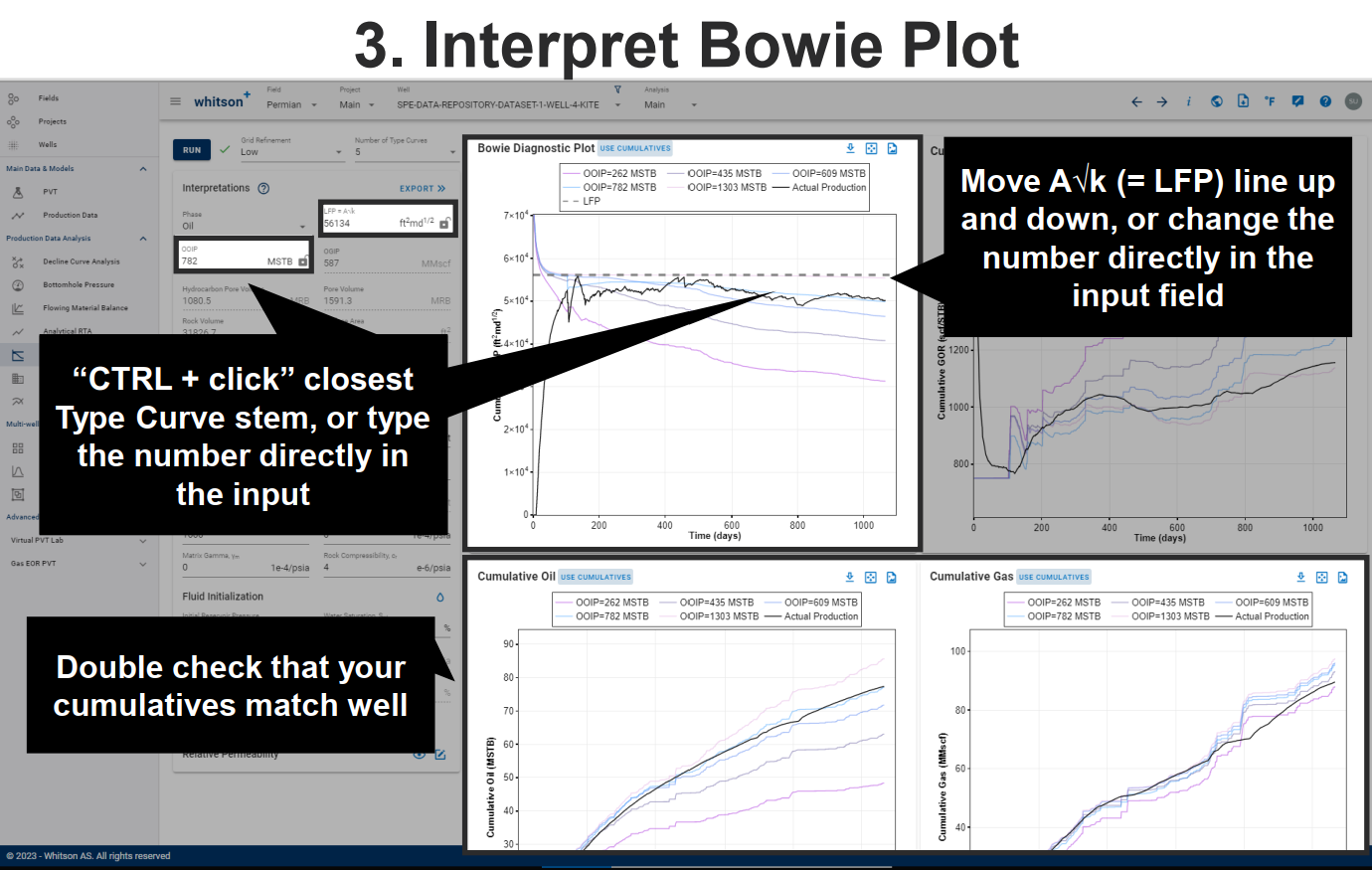
- Pick a “Representative LFP'” based on the early time “LFP'” plot. Remember that a flat, horizontal line is expected during infinite acting behavior.
- Multiply each the LFP'/OOIP ratios simulated in Step 5 by the “Representative LFP'” picked in Step 6.
- Pick the OOIP stem that matches the actual production data the best.
3. Numerical RTA workflow in whitson+
The Numerical RTA workflow presented above is fully automated in whitson+, and is split into three steps, manifesting one of the key benefits of the workflow, i.e. decoupling of multi-phase flow related data (PVT, initial saturations and relative permeabilities) from well geometry and petrophysical properties (\(L_w\) , \(x_f\), h, \(N_f\) , \(\phi\), \(k\) ).
3.1. Step 1. Fluid Initialization and Relative Permeability
Before running the numerical RTA workflow, a relevant fluid initialization and relative permeability set must be assigned to the well of interest. The fluid initialization part involves assigning a representative in-situ fluid for the hydrocarbon phase (i.e. GOR) and initial water saturation.
Make sure to run the infinite acting case for this set of input parameters before continuing to step 2 to ensure that the producing GOR and water cut performance makes sense, i.e.:
- Simulated producing GOR must be (about) equal to or less than the actual GOR. The GOR of the infinite acting model should never be higher than the actual GOR.
- Mismatch between the observed water cut and the simulated water cut is as small as possible. Some mismatch during the early time (during flowback) is expected. Water cut is not very sensitive to flow regime so one should not expect a major change in water cut when entering boundary dominated flow.
3.2. Step 2. Pick LFP' and OOIP
With the fluid initialization and relative permeability curves from Step 1, generate type curves, and pick a representative LFP' and OOIP based on the different diagnostic plots. With real data, it can be helpful to use several diagnostic plots to home in on a good, final result. If the match of both cum oil and cum gas is satisfactory, e.g. if the Bowie plot, cumulative oil and cumulative gas plot indicate different OOIPs, it might be required to go back and redo step 1. If satisfactory results are obtained, move forward to step 3.
3.3. Step 3. Resolve parameters for history matching
Input estimates for porosity, well lateral length, number of fractures and reservoir height to resolve estimates for permeability and fracture half length. If wanted, these parameters can be exported to the history matching module for further analysis (upon export to the history matching module, the first run should yield a good match of the observed production data).
4. Info About the "Template Model"
The "template model" referred to in the numerically assisted RTA workflow described above and used in whitson+ is different if the \(F_{cd}\) is above or below 500. When \(F_{cd}\) > 500 we treat the fracture as infinite conductive, and we use smaller template model, and less grid cells in x-direction, to make the model run faster. When \(F_{cd}\) < 500 the pressure drop in the fracture becomes increasingly more important as the has the \(F_{cd}\) gets smaller. Hence, a larger template model, with more grid cells in the x-direction, is used to capture pressure drop across the fracture surface. Below is a summary of the input parameters for the two different template models.
| Dimension | Symbol | < 500 | > 500 |
|---|---|---|---|
| Lateral Length | Dynamic | Dynamic | |
| Reservoir Half-Extent | 400 ft | 25 ft | |
| Fracture Half-Length | 400 ft | 25 ft | |
| Fracture Height | 200 ft | 12.5 ft | |
| Reservoir Height | 200 ft | 12.5 ft | |
| No. of Fractures | 1 | 1 | |
| Matrix Permeability | 200 nd | 200 nd | |
| Porosity | 0.05 | 0.05 |
For the smaller OOIPs mentioned in step 5 here, the only parameter that change from the template model is \(L_w\), where each smaller OOIP corresponds to a \(L_w\) of 100 ft, 90 ft, 80 ft, 70 ft, 60 ft, 50 ft, 40 ft, 30 ft, 20 ft.
There must always be a case that's infinite acting. The size of that model is dynamically set to be \(L_w = max(500, 60 + 50 \times\) .
5. Significance of the shape of Bowie Diagnostic Plot
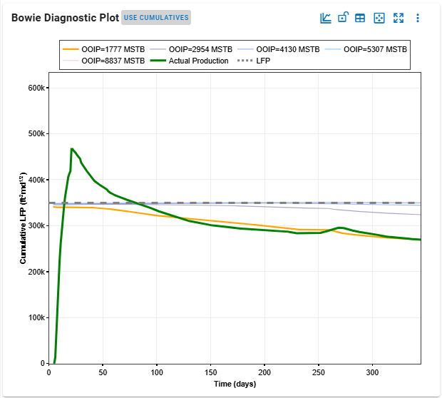
The green line in the Bowie plot is following the actual production data. If the shape of your actual production data matches 1-to-1 with the outputs of the model, the line would be flat. However, the production data we have in the field is rarely perfect, and this is where the differences come up. The way the green line is calculated is explained in detail in the manual here.
Sometimes, very early-time data can be ignored due to flowback effects and other operational changes (such as casing-to-tubing flow) that induce non-reservoir effects.
Additionally, very early-time data may exhibit bilinear flow, which can significantly impact overall well deliverability. Adjusting parameters such as fracture conductivity, and fracture and matrix permeability can influence the position of the green line in the Bowie diagnostic plot. Furthermore, the initial reservoir pressure can also significantly impact the shape of the Bowie plot.
We recommend watching this video to learn more about the shape of the LFP plot:
You can also download the presentation here
6. Time-stepping, number and relative Sizes of Type Curves
You can pick between running 5 and 10 type curves. Each type curve represents an individual numerical simulation run, with its associated pore volume. In other words, it dictates if you'll see 5 or 10 stems (in addition to the actual production data) in the different Numerical RTA plots. The smaller option (e.g. "5 smaller models") divides the \(L_w\) in the template model by 2. The larger option (e.g. "5 larger models") multiplies all the \(L_w\) in the template model by 2.
The BHP and grid refinement is used to run the simulation model and Time-Stepping dictates how many timesteps should be passed to the simulator.
Higher number of time-steps takes longer to run since the simulator tries to match the BHP for all these time steps. A significant reduction of the model run-times can be achieved with a negligible trade off in model accuracy - which is especially useful for wells with long, noisy producing history or BHP. Here are the available options to control the number of timesteps to use for simulation:
| Timestep Option | Description |
|---|---|
| All | Simulates every uploaded timestep. |
| Smart | Simulates daily timesteps for the first 100 days and then every 10th point after that. |
| Custom | Simulates every Nth timestep, where you can specify 'N'. Example if you set N=7, the simulator simulates weekly timesteps. |
7. LFP Differences between Analytical, Fractional and Numerical RTA
Numerical RTA generally yields a greater LFP value compared to Analytical RTA.
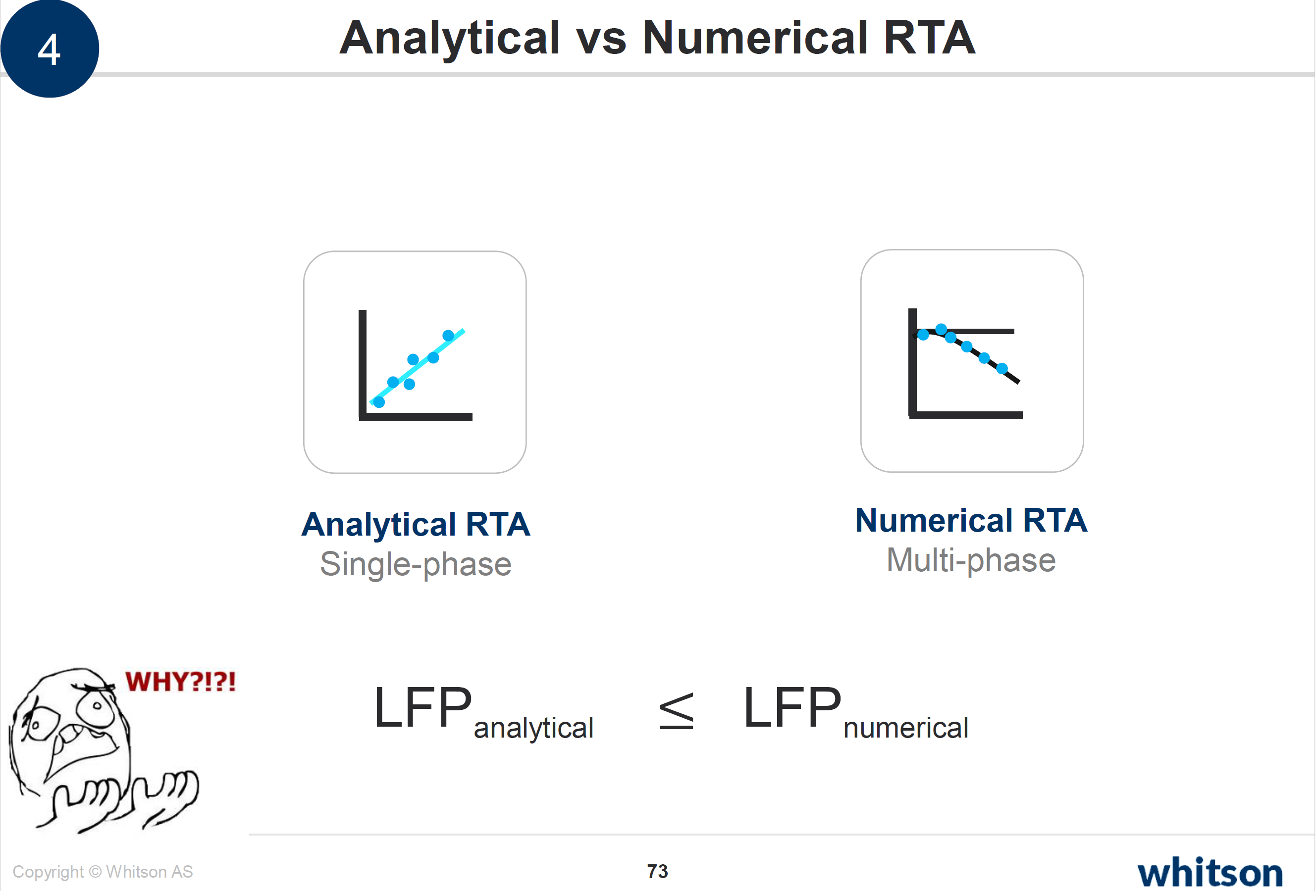
Given that each technique calculates LFP slightly differently, comparisons of LFP values should be made between wells using the same technique.
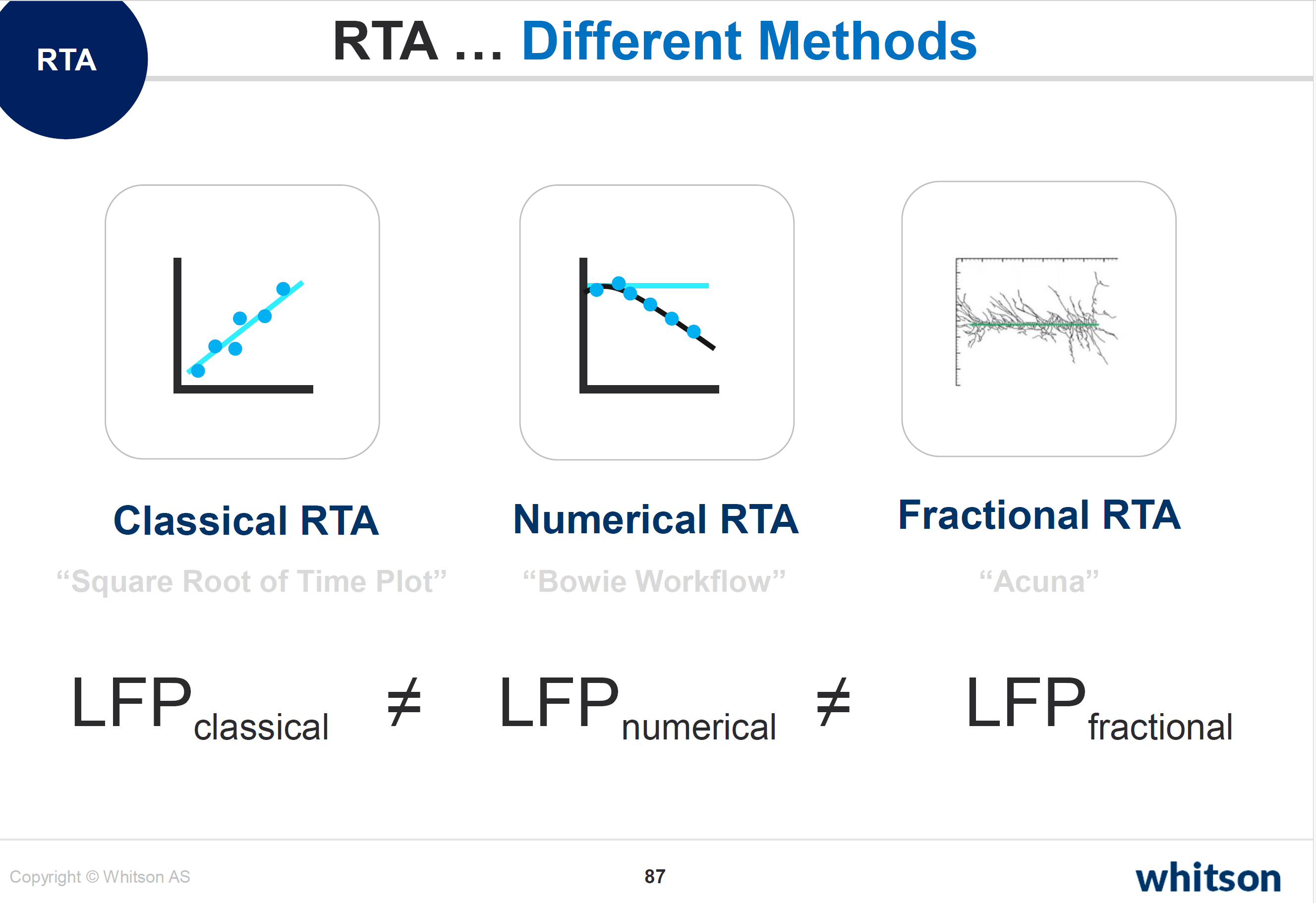
The differences between analytical, fractional and numerical RTA, are due to the following factors:
| Method | How LFP is Derived |
|---|---|
| Analytical RTA | LFP is derived from 'single-phase' and graphical picks from the square root time plot. The equations in Section 1.11 demonstrate the calculation of LFP from the slope and it's crucial to note that this calculation relies on 'initial PVT properties'. |
| Fractional RTA | LFP is derived using a similar method (graphical slope selection for delta) and calculates LFP as \(Ak^\delta\), not \(Ak^{0.5}\). The equations used for the LFP calculation are available here . |
| Numerical RTA | LFP is calculated very differently compared to the two techniques above. It is derived from a scaling of the LFP of the underlying template model used to generate the different simulated finite-acting and infinite-acting stems. You can find the numerical RTA LFP calculation workflow here . |
You can find more information and an example where a numerical model is run and the results are plugged in as input into the analytical RTA solutions in this slide deck here.
8. Benefits with the Numerical RTA Workflow
The numerical RTA workflow proposed by Bowie and Ewert (2020) has the following benefits:
- First, it solves the inherent problems associated with rigorous superposition and multiphase flow effects involving time and spatial changes in pressure, compositions and PVT properties, saturations and complex phase mobilities.
- The Numerical RTA workflow decouples multi-phase flow data (PVT, initial saturations and relative permeabilities) from well geometry and petrophysical properties (\(L_w\), \(x_f\), \(h\), \(N_f\), \(\phi\), \(k\)), providing a rigorous yet rapid and semi-automated approach to define production performance for many wells.
- Semi-analytical models, time and spatial superposition (convolution), pseudopressure and pseudotime transforms are not required.
- The method has proven to increase the consistency between engineers in a team compared to traditional RTA methods (URTeC 2967).
- The speed and repeatability of the method still allows for many wells to be analyzed efficiently.
- The fact that the method utilizes a full-physics numerical model, makes it a trivial exercise to export the results from the RTA analysis into higher order analysis such as a full-physics reservoir and associated history matching.
9. Finite Conductivity Fractures
When \(F_{cd}\) is inputed lower than 500 in the Numerical RTA workflow, the \(F_{cd}\) conversion outlined below is leveraged when exporting the results to the history matching module.
9.1. Consistently Changing \(F_{cd}\) when other Parameters Change
Sometimes an additional pressure drop in the fracture might be required to match historical observed data (e.g. GOR performance), and this can be included in the model by assigning a low dimensionless fracture conductivity (\(F_{cd}\)) to the model at hand. The lower the \(F_{cd}\), the higher the pressure drop in the fracture. A finite conductivity fracture is typically associated with a linear GOR increase when the flowing bottomhole pressure is below the saturation pressure.
The physical reasons for this additional pressure drop can be many, but numerically the low \(F_{cd}\) will in the end of the day be just that, an additional pressure drop between the reservoir and the well. Wells that exhibit this behavior might qualify as good clean-up candidates.
To consistently incorporate a finite conductivity fracture into the numerically assisted RTA workflow, one needs to know how the definition of dimensionless fracture conductivity \(F_{cd}\) changes when other parameters change (e.g. permeability, height, number of fractures).
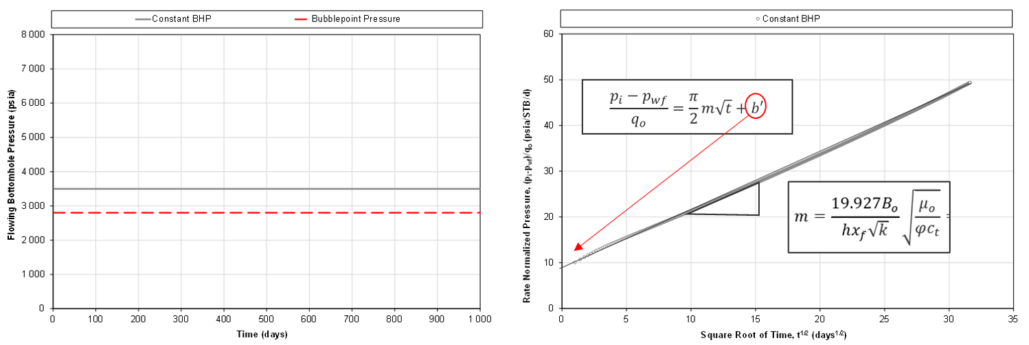
Fig. 3: Example of square root of time plot for finite conductive fracture.
For an ideal model (e.g. single-phase flow, controlled on a constant bottomhole pressure), linear flow associated with flow through an finite conductive fracture manifests itself as a positive intercept on the square root of time plot, as exemplified in Fig. 3.
For a well with a given slope m (which is a composite of the LFP' and PVT related parameters), the intercept should be the same no matter what combination of parameters that make up m, i.e. irrespective of LFP'. Hence, one can convert \(F_{cd}\) consistently from with the following relationship:
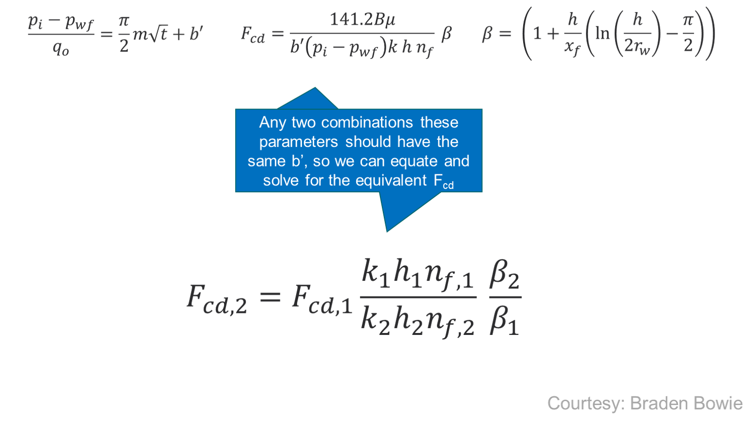
An excel file with the relationships coded up can be obtained here. In whitson+, the \(F_{cd}\) conversion is activated when the inputed \(F_{cd}\) is lower than 500. Relevant for this conversion are the following parameters in the "template model".
| Dimension | Symbol | Default Value |
|---|---|---|
| Well Radius | \(r_w\) | 1 ft |
| Fracture Half-Length | \(x_f\) | 400 ft |
| Reservoir Height | \(h\) | 200 ft |
| No. of Fractures | \(N_f\) | 1 |
| Matrix Permeability | \(k\) | 200nd |
9.2. Impact of \(x_{f}\)/h ratio
When verifying the relationships mentioned above with a numerical reservoir simulation model, it was found that the results hold as long as the \(x_{f}\)/h ratio in the "template model" and a given realization is the same. This is exemplified in Fig. 5.
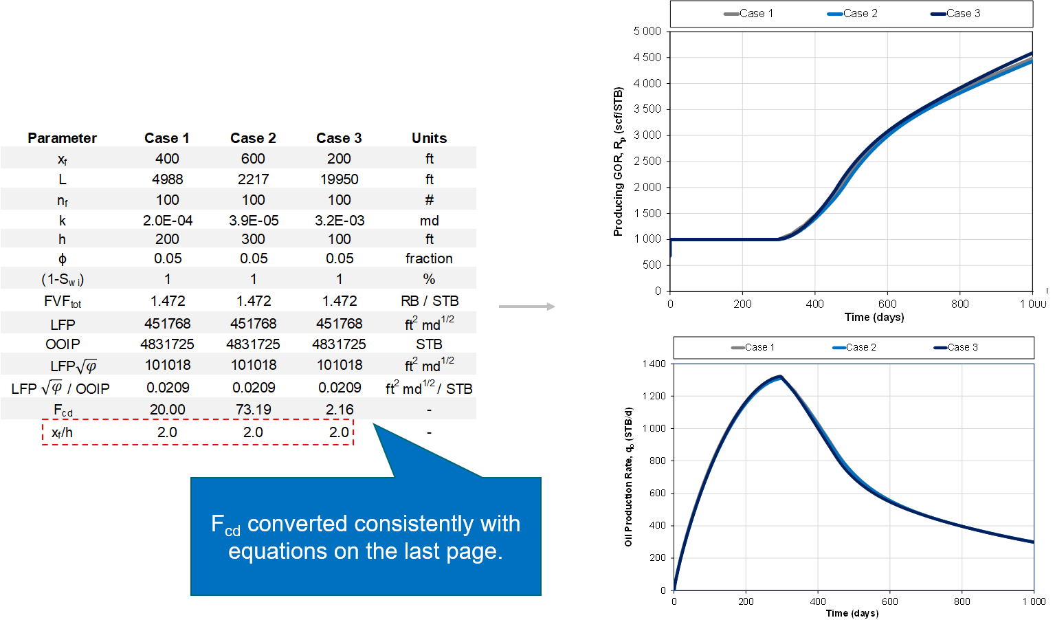
Fig. 5: Same \(x_{f}\)/h ratio
However, if the \(x_{f}\)/h between the "template model" and a given realization is different, then the GOR behavior will not be identical, as exemplified in Fig. 6.
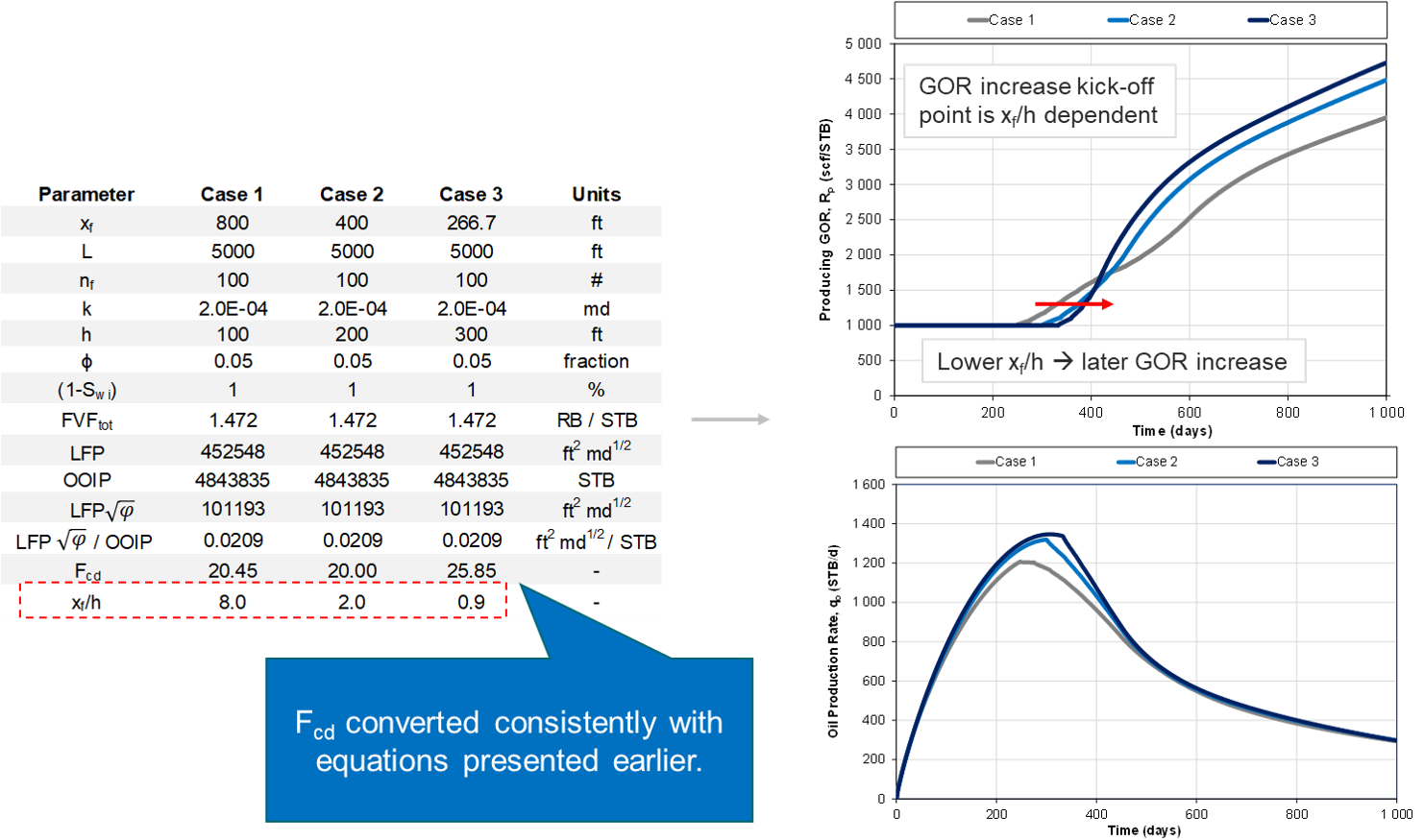
Fig. 6: Different \(x_{f}\)/h ratio
Implementation of \(x_{f}\)/h ratio in whitson+
As of right now, it is not possible to input a pre-defined \(x_{f}\)/h into the numerical RTA workflow whitson+, but if you will like us to implement that, let us know. We are also interested to hear from you if you have an elegant way of solving the consistent conversion of \(F_{cd}\) without requiring \(x_{f}\)/h as an input.
10. Numerical RTA accounting for Uneven Frac Spacing
An inherent assumption in most industry RTA is equally spaced fractures. However, as shown in several field studies (Raterman 2017, Gale 2018), the distance between individual fractures tends to be unevenly spaced along the wellbore (e.g. “fracture swarms”). Below, we extend the original numerical RTA workflow to account for uneven fracture spacing.
10.1. Flow Regimes
To understand why it is important to account for uneven fracture spacing, we repeat the three relevant flow regimes tight unconventionals.
| Flow Regimes | Description |
|---|---|
| Infinite Acting Flow | Often referred to as transient flow, is the flow regime that ends as the pressure transient reaches one reservoir boundary. |
| Transitional Flow | This the flow regime starts as the pressure transient reaches one reservoir boundary and ends when the pressure propagation reaches all reservoir boundaries. |
| Boundary Dominated Flow (\(\frac{\partial p}{\partial t}= \) constant at all locations) | Also called pseudo-stedy state, is the flow regime that starts as the pressure propagation reaches all reservoir boundaries. It occurs when all outer boundaries of the reservoir are no-flow boundaries. These boundaries can be both sealing faults and nearby producing wells or fractures. During this period, the change in pressure at any place in the reservoir decreases at the same, constant rate. The reservoir is said to behave as a “tank”. |
For a well geometry with uneven fracture spacing, the flow regime is (1) infinite acting until the boundary between the fractures with the smallest spacing is observed, (2) thereafter it is transitional flow until the boundary between the fractures with the largest spacing is observed, and (3) after that it is in full boundary dominated flow.
10.2. Key underlying assumption in classical RTA - 1D Reservoir Model
Traditional RTA methods leverage a so-called "symmetry element" model, in which the underlying model is representing one-quarter of a fracture. This is highlighted by the red-lined box in Fig. 1. The model is “1 dimensional”, as there are no flow contributions beyond the fractips (\(x_{f}\) = \(x_{e}\)) or beyond the frac height (\(h_{f}\) = \(h\)). Hence, there is only one no-flow boundary, resulting in only two dominant flow regimes over time; (1) infinite acting (IA) linear flow, followed by (2) boundary dominated (BD) flow.
The problem with this model when applied to real field cases is that all observed boundary effects are “forced” into one boundary (which is observed at one point in time). However, as shown in several field studies (Raterman 2017, Gale 2018), the distance between individual fractures tends to be unevenly spaced along the wellbore, resulting in boundaries being observed at different points in time. The resulting well performance is a compound result of observing different reservoir boundaries (here fractures) at different points in time. Hence, characterizing and accounting for transitional flow becomes important . Transitional flow can in many cases be the dominant flow regime for unconventional wells, especially if the fracture spacing is highly uneven (high heterogeneity).
10.3. Numerical RTA with Uneven Fracture Spacing: Key Geometric Variables
To understand the numerically assisted RTA workflow outlined in this paper, the theoretical background must be presented and validated. To reduce the number of geometric variables, the generalized, linear flow parameter (LFP’) and original oil in place (OOIP) are defined as follows to account for all values of
For a given porosity, one can observe that the generalized LFP (LFP') is simplified to the familiar LFP=A√k.
10.4. Relationship between , LFP’ and OOIP
For a given fluid initialization (PVT and \(S_{wi}\)), relative permeability curves, and bottomhole-pressure profile versus time, wells with the same , LFP’ and OOIP yield the same well performance for all times and all flow regimes. In other words, if , LFP’ and OOIP are the same, the well performance is identical (rates, cumulatives, GOR, water cuts), independent of time and flow regime. This fundamental relationship is exemplified Fig. 7. This provides the foundation for numerical RTA, and lead to an efficient, semi-automated process to perform rigorous RTA, even for more complex geometries.
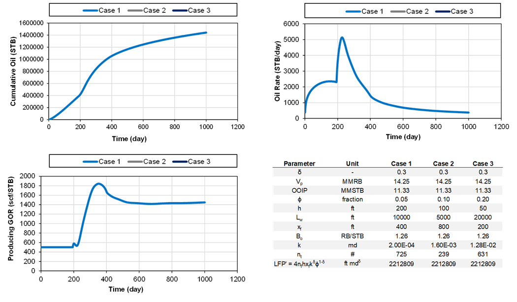
Fig. 7: Example of three different cases with the same , LFP’ and OOIP (all overlapping).
10.5. Simple Construction of a Reservoir Model with Uneven Fracture Spacing
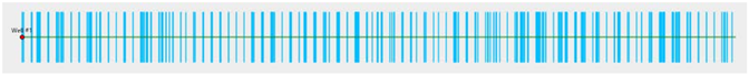
Fig. 8: Example of network with parallel fractures with uneven spacing (Acuna 2020).
The parameter represents a distribution of uneven frac spacings (S=2\(y_{e}\))), as exemplified in Fig. 8. Once a given has been characterized (e.g., by leveraging the diagnostic plot in the analytical RTA feature), one can create a distribution of different symmetry of element models, each with a different distance (\(y_{e}\)) to the closest boundary (parallel fractures with different spacing also called a fracture “swarm” geometry), to represent this parameter. This is done in the following steps
- Pick some arbitrary reservoir parameters for a “template” model, e.g., φ=0.05, h = 200 ft, \(L_{w}\) = 10000 ft, \(x_{f}\) = 400 ft and k = 200 nd. Calculate the associated contacted pore volume (\(V_{p}\)=\(2L_{w}x_{f}hφ\) ).
- Select a maximum and minimum frac-to-frac spacing (\(S_{min}\) and \(S_{max}\)), e.g., \(S_{min}\) = 2 ft and \(S_{max}\) = 50 ft.
- Select a number of different fragment sizes, m.
-
Each fragment size has its own frac-to-frac spacing (\(S_{i}\)). Calculate the ratio, R, between each fragment size
-
Let \(n_{1}\) be the number of fragments of size \(S_{max}\). The number of fragments n_i with size greater or equal to (\(S_{i}\)) is given by
This relationship is valid for all sizes except the smallest one because this size must compensate for the absence of sizes smaller than \(S_{min}\).
-
Calculate \(x_{mf}\) by
-
Calculate the total number of fragments \(n_{t}\)
-
Calculate the number of fragments of maximum size \(n_{1}\) with

10.6. Numerical RTA with Uneven Fracture Spacing ( parameter)
The original numerical RTA workflow is modified as follows to account for uneven fracture spacing
- Create m number (e.g. m = 10) of symmetry of element models (“template models”) with each having its own fracture-to-fracture distance \(S_{i}\) (i.e. different OOIP and OGIP) according to the process outlined in the previous section.
- The fragment size \(S_{i}\) of the different symmetry of element models is not a function of delta, just \(S_{min}\), \(S_{max}\) and m as given by Eq. \ref{eq:R}. Hence, an estimate of is not required for this step.
- The largest numerical symmetry element model should be large enough to behave infinite acting (=large OOIP) for the entirety of the historical time of the well being analyzed, while the smallest one should observe boundary effects within a few days of productions.
- In practice, this entails creating m number of single-fracture, numerical models with the same h, \(x_{f}\), k and φ, same fluid initialization (PVT and \(S_{wi}\)) and relative permeability relations. The only thing that is different for the different models is the fracture-to-fracture distance (or fragement size), \(S_{i}\).
- Run all the individual models individually (can be done in parallel) controlled by (a) the wells’ actual measured bottomhole pressure, and (b) zero rate during shut-ins.
- Use the diagnostic plot given in the analytical RTA module to estimate . This is just a starting point and can be changed easily later without having to rerun the numerical models.
- Use the estimate of and the process provided in the previous section to come up with the number of each fragment size that should make up the total production. In other words, estimate the number \(n_{i}\) of each fragment size \(S_{i}\).
- Calculate the total LFP’ and total OOIP for this model as given by Eq. 2 and Eq. 3
- Calculate the total simulated production with a sumproduct, e.g. \(q_{o,sim}=∑ n_i q_{o,i}\).
- Calculate the ratio between the actual measured oil rates and the total simulated model oil rates: \(r=q_{o,actual}/q_{o,sim}\). Alternatively, one can use the cumulative to reduce noise: \(r=Q_{o,actual}/Q_{o,sim}\).
- Calculate the daily LFP' by multiplying the daily ratio r (Step 7) with the known LFP' of the simulated case (Step 5).
- a horizontal flat line indicates infinite acting or transitional flow
- deviation below this line represents boundary dominated flow (also called end of characteristic flow by Acuna 2016).
- the magnitude of the horizontal trend indicates the LFP'.
- Pick a “Representative LFP'” based on the early time of the LFP' plot.
- At this point it can also be relevant to change to see what effect it has on the diagnostic plot (it is quick as it does not require rerunning the models, just replotting the data).
- Repeat the steps 1-10 for multiple, smaller OOIP volumes (reduce the size of \(S_{max}\) in the "template model"). This results in several “type curves” with each its own LFP'/OOIP ratio .
- Multiply each LFP'/OOIP ratio simulated in Step 11 by the “Representative LFP'” picked in Step 9.
- Pick the OOIP stem that best matches the actual production data the best.
11. How to Handle Simulation of Different pRi and GORi?
The black-oil PVT table is always generated in whitsonʳˢ from initial composition (), reservoir temperature (), equation of state (EOS), and surface process configuration. The black-oil PVT table is always regenerated locally at runtime, taking only a fraction of a second. This approach ensures flexibility and avoids delays previously encountered when downloading pre-generated BOT files from the cloud.
Current handling for variations in initial reservoir pressure () and initial GOR ():
The black-oil PVT table is primarily a function of (through ) and (). The is used to initialize the fluid as either single-phase or two-phase. This parameter is not a direct input in the generation of the black-oil PVT table but is used during its extrapolation to avoid numerical instabilities of negative compressibility and internal extrapolation as much as possible. Therefore, the extrapolated part of the black-oil PVT table (affected by ) is typically outside the region used in simulations and should not materially impact the quality of the results.
-
Variations in with fixed
When is held constant, the same is used across all cases. Varying influences the initialization of the fluid system:
- If > , the fluid initializes as single-phase.
- If ≤ , the fluid initializes as two-phase.
Effect of on History Matching
If you compare the files of two History Matching cases with same , but different , there may also be some differences in the extrapolated part of the black-oil PVT table, but that should not impact the simulations.
-
Variations in with fixed
Changing is equivalent to altering the . For each case, black-oil PVT table will be generated using different composition. A new composition () is generated by taking the original obtained from Fluid Definition and recombining it to match the specified . A new BOT is then constructed based on () and used in the simulation.
-
Variations in both and
Both effects described in previous points are applied simultaneously.
References
[2] Acuña, J.A. 2020. Rate Transient Analysis of Fracture Swarm Fractal Networks. Paper URTeC 2118.