Recovery Factor Analysis

1. Theory

Recovery Factor Analysis forecasts future fluid rates by extending the straight-line trend obtained from the multiphase flowing material balance (FMB) analysis. The forecast assumes that future production behavior continues to honor the established FMB trend.

The calculation is performed on time-step basis. At each forecast step, the method solves a quadratic equation for the predicted gas rate ($q_g$). The predicted oil and water rates are then calculated using the forecasted instantaneous oil-gas ratio ($ogr$) and water-gas ratio ($wgr$). Once the phase rates are known, cumulative oil, gas, and water production can be updated, and recovery factors can be calculated from the corresponding original hydrocarbons in place.

1.1. Requirements

Recovery Factor Analysis requires a completed multiphase FMB analysis. The following inputs are required:

1. Contacted pore volume ($V_p$) and multiphase productivity index ($b_M$) from the multiphase FMB analysis.
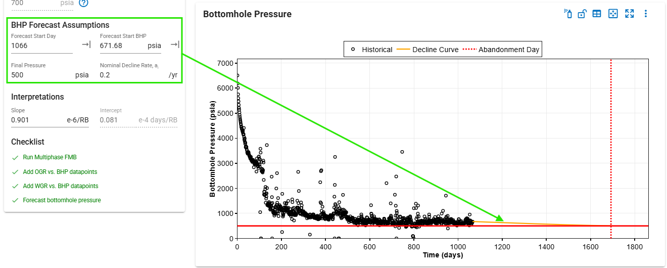
2. A forecast of flowing bottomhole pressure ($p_{wf}$) versus time.
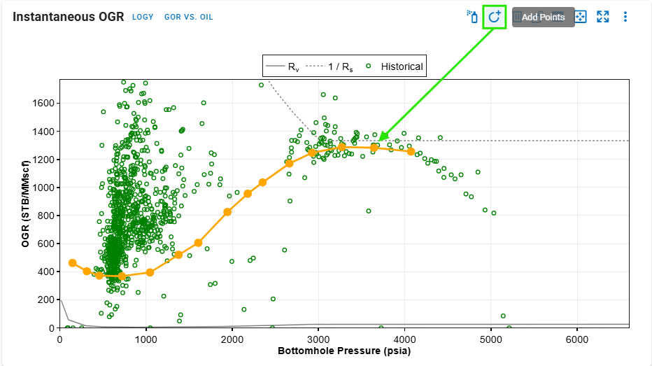
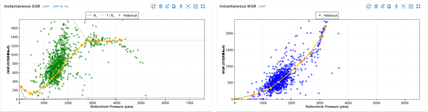
3. A forecast of instantaneous flowing oil-gas ratio ($ogr$) versus $p_{wf}$.
4. A forecast of instantaneous flowing water-gas ratio ($wgr$) versus $p_{wf}$.

The flowing $ogr$ and $wgr$ trends are generated from the multiphase FMB analysis and extrapolated over the forecast pressure range.

1.2. Quadratic Equation Derivation

The derivation starts from the cumulative producing oil-gas ratio ($OGR$) and water-gas ratio ($WGR$) at day (t+1),

$$\begin{equation} \label{Cum-OGR} % (STB/Mscf) OGR^{t+1}=\frac{N_p^{t+1}}{G_p^{t+1}}=\frac{N_p^{t}+ogr^{t+1}q_g^{t+1}}{G_p^{t}+q_g^{t+1}} \end{equation}$$

$$\begin{equation} \label{Cum-WGR} % (STB/Mscf) WGR^{t+1}=\frac{W_p^{t+1}}{G_p^{t+1}}=\frac{W_p^{t}+wgr^{t+1}q_g^{t+1}}{G_p^{t}+q_g^{t+1}} \end{equation}$$

Please note that uppercase $OGR$ and $WGR$ represent cumulative producing ratios, while lowercase $ogr$ and $wgr$ represent instantaneous flowing ratios.

As described in the multiphase FMB section, cumulative producing ratios can also be expressed in terms of component concentrations,

$$\begin{equation} \label{Cum-OGR-MFMB} % (STB/Mscf) OGR^{t+1}=\frac{\zeta_{oi}-\left(\frac{S_o^{t+1}}{B_o^{t+1}}+\frac{S_g^{t+1}R_v^{t+1}}{B_g^{t+1}}\right)}{\zeta_{gi}-\left(\frac{S_o^{t+1}R_s^{t+1}}{B_o^{t+1}}+\frac{S_g^{t+1}}{B_g^{t+1}}\right)} \end{equation}$$

$$\begin{equation} \label{Cum-WGR-MFMB} % (STB/Mscf) WGR^{t+1}=\frac{\zeta_{wi}-\left(\frac{S_w^{t+1}}{B_w^{t+1}}\right)}{\zeta_{gi}-\left(\frac{S_o^{t+1}R_s^{t+1}}{B_o^{t+1}}+\frac{S_g^{t+1}}{B_g^{t+1}}\right)} \end{equation}$$

where the component concentrations of oil ($\zeta_o$), gas ($\zeta_g$), and water ($\zeta_w$) are defined as:

$$\begin{equation} \label{Component-Concentration-Oil} % (STB/bbl) \zeta_{o}=\frac{S_o}{B_o}+\frac{S_gR_v}{B_g} \end{equation}$$

$$\begin{equation} \label{Component-Concentration-Gas} % (Mscf/bbl) \zeta_{g}=\frac{S_oR_s}{B_o}+\frac{S_g}{B_g} \end{equation}$$

$$\begin{equation} \label{Component-Concentration-Water} % (STB/bbl) \zeta_{w}=\frac{S_w}{B_w} \end{equation}$$

Subscripts $o$, $g$, and $w$ represent oil, gas, and water properties; while subscript $i$ is for initial condition. Definitions and units for all variables can be seen in the Nomenclature.

Combining these two definitions results in: $$\begin{equation} \label{Cum-OGR-Combined} % (STB/Mscf) \frac{N_p^{t}+ogr^{t+1}q_g^{t+1}}{G_p^{t}+q_g^{t+1}}=\frac{\zeta_{oi}-\left(\frac{S_o^{t+1}}{B_o^{t+1}}+\frac{S_g^{t+1}R_v^{t+1}}{B_g^{t+1}}\right)}{\zeta_{gi}-\left(\frac{S_o^{t+1}R_s^{t+1}}{B_o^{t+1}}+\frac{S_g^{t+1}}{B_g^{t+1}}\right)} \end{equation}$$

$$\begin{equation} \label{Cum-WGR-Combined} % (STB/Mscf) \frac{W_p^{t}+wgr^{t+1}q_g^{t+1}}{G_p^{t}+q_g^{t+1}}=\frac{\zeta_{wi}-\left(\frac{S_w^{t+1}}{B_w^{t+1}}\right)}{\zeta_{gi}-\left(\frac{S_o^{t+1}R_s^{t+1}}{B_o^{t+1}}+\frac{S_g^{t+1}}{B_g^{t+1}}\right)} \end{equation}$$

Total saturation is denoted by:

$$\begin{equation} \label{Saturation} S_o^{t+1}+S_g^{t+1}+S_w^{t+1}=1 \end{equation}$$

Combining the production-based ratio definitions with the component-concentration definitions allows oil and water saturation to be written as functions of the unknown gas rate ($q_g^{t+1}$) by rearranging Eq. \eqref{Cum-OGR-Combined} and Eq. \eqref{Cum-WGR-Combined}.

$$\begin{equation} \label{Oil-Saturation} % (-) S_o^{t+1}=\frac{A_o^{t+1}q_g^{t+1}+C_o^{t+1}}{A_d^{t+1}q_g^{t+1}+C_d^{t+1}} \end{equation}$$

$$\begin{equation} \label{Water-Saturation} % (-) S_w^{t+1}=\frac{A_w^{t+1}q_g^{t+1}+C_w^{t+1}}{A_d^{t+1}q_g^{t+1}+C_d^{t+1}} \end{equation}$$

where the constants are:

$$\begin{equation} \label{Ao} A_o^{t+1}=B_o^{t+1}\left[\zeta_{gi}\left(B_g^{t+1}ogr^{t+1}+B_w^{t+1}R_v^{t+1}wgr^{t+1}\right)-\zeta_{oi}\left(B_g^{t+1}+B_w^{t+1}wgr^{t+1}\right)+\left(ogr^{t+1}-R_v^{t+1}\right)\left(\zeta_{wi}B_w^{t+1}-1\right) \right] \end{equation}$$

$$\begin{equation} \label{Aw} A_w^{t+1}=B_w^{t+1}\left\{wgr^{t+1}\left[\zeta_{gi}\left(B_g^{t+1}-B_o^{t+1}R_v^{t+1}\right)+\zeta_{oi}\left(B_o^{t+1}-B_g^{t+1}R_s^{t+1}\right)-\left(1-R_s^{t+1}R_v^{t+1}\right) \right]\\+\zeta_{wi}\left[ogr^{t+1}\left(B_g^{t+1}R_s^{t+1}-B_o^{t+1}\right)+B_o^{t+1}R_v^{t+1}-B_g^{t+1} \right]\right\} \end{equation}$$

$$\begin{equation} \label{Ad} A_d^{t+1}=B_g^{t+1}\left(ogr^{t+1}R_s^{t+1}-1\right)+B_o^{t+1}\left(R_v^{t+1}-ogr^{t+1}\right)+B_w^{t+1}wgr^{t+1}\left(R_s^{t+1}R_v^{t+1}-1\right) \end{equation}$$

$$\begin{equation} \label{Co} C_o^{t+1}=B_o^{t+1}\left[\zeta_{gi}\left(B_g^{t+1}N_p^{t}+B_w^{t+1}R_v^{t+1}W_p^t\right)-\zeta_{oi}\left(B_g^{t+1}G_p^t+B_w^{t+1}W_p^t\right)+\left(N_p^t-G_p^tR_v^{t+1}\right)\left(\zeta_{wi}B_w^{t+1}-1\right) \right] \end{equation}$$

$$\begin{equation} \label{Cw} C_w^{t+1}=B_w^{t+1}\left\{W_p^t\left[\left(R_s^{t+1}R_v^{t+1}-1\right)-\zeta_{gi}\left(B_o^{t+1}R_v^{t+1}-B_g^{t+1}\right)-\zeta_{oi}\left(B_g^{t+1}R_s^{t+1}-B_o^{t+1}\right) \right]\\+\zeta_{wi}\left[B_g^{t+1}\left(N_p^tR_s^{t+1}-G_p^t\right)-B_o^{t+1}\left(N_p^t-G_p^tR_v^{t+1}\right) \right]\right\} \end{equation}$$

$$\begin{equation} \label{Cd} C_d^{t+1}=N_p^t\left(B_g^{t+1}R_s^{t+1}-B_o^{t+1}\right)+G_p^t\left(B_o^{t+1}R_v^{t+1}-B_g^{t+1}\right)+W_p^tB_w^{t+1}\left(R_s^{t+1}R_v^{t+1}-1\right) \end{equation}$$

After expressing $S_o^{t+1}$ and $S_w^{t+1}$ as functions of $q_g^{t+1}$. These expressions are then substituted into the mixture-density equation.

$$\begin{equation} \label{Mixture-Density} % lbm/bbl \beta=5.615\rho_{o,sc}\left(\frac{S_o}{B_o}+\frac{S_gR_v}{B_g}\right)+1000\rho_{g,sc}\left(\frac{S_oR_s}{B_o}+\frac{S_g}{B_g}\right)+5.615\rho_{w,sc}\left(\frac{S_w}{B_w}\right) \end{equation}$$

Subscript $sc$ indicates standard condition. Substituting $S_o$ and $S_w$ in Eq. \eqref{Mixture-Density} with Eqs. \eqref{Oil-Saturation} and \eqref{Water-Saturation} in terms of $q_g^{t+1}$ yields:

$$\begin{equation} \label{Beta} \beta^{t+1}=\frac{D^{t+1}q_g^{t+1}+E^{t+1}}{B_g^{t+1}B_o^{t+1}B_w^{t+1}\left(A_d^{t+1}q_g^{t+1}+C_d^{t+1}\right)} \end{equation}$$

where,

$$\begin{equation} \label{D} D^{t+1}=\alpha_g^{t+1}A_d^{t+1}B_o^{t+1}B_w^{t+1}+A_w^{t+1}B_o^{t+1}\left(\alpha_wB_g^{t+1}-\alpha_g^{t+1}B_w^{t+1}\right)\\+A_o^{t+1}B_w^{t+1}\left(\alpha_o^{t+1}B_g^{t+1}-\alpha_g^{t+1}B_o^{t+1}\right) \end{equation}$$

$$\begin{equation} \label{E} E^{t+1}=B_g^{t+1}\left(\alpha_wB_o^{t+1}C_w^{t+1}+\alpha_o^{t+1}B_w^{t+1}C_o^{t+1}\right)+\alpha_g^{t+1}B_o^{t+1}B_w^{t+1}\left(C_d^{t+1}-C_o^{t+1}-C_w^{t+1}\right) \end{equation}$$

$$\begin{equation} \label{alpha-g} \alpha_g^{t+1}=5.615\rho_{o,sc}R_v^{t+1}+1000\rho_{g,sc} \end{equation}$$

$$\begin{equation} \label{alpha-o} \alpha_o^{t+1}=5.615\rho_{o,sc}+1000\rho_{g,sc}R_s^{t+1} \end{equation}$$

$$\begin{equation} \label{alpha-w} \alpha_w=5.615\rho_{w,sc} \end{equation}$$

Next, recall the multiphase FMB equation at day $t+1$:

$$\begin{equation} \label{Multiphase-FMB} \frac{\beta_i-\beta^{t+1}}{\dot{m}^{t+1}}=\frac{1}{V_p}{MBT}_M^{t+1}+\frac{1}{b_M} \end{equation}$$

$MBT_M$ is the mass material balance time,

$$\begin{equation} \label{Mass-Material-Balance} % day {MBT}_M^{t+1}=\frac{M_T^{t+1}}{\dot{m}^{t+1}} \end{equation}$$

The mass flow rate is calculated as:

$$\begin{equation} \label{Total-Mass-Production} % lbm/d \dot{m}^{t+1}=5.615\rho_{o,sc}q_o^{t+1}+1000\rho_{g,sc}q_g^{t+1}+5.615\rho_{w,sc}q_w^{t+1}\\=q_g^{t+1}\left(5.615\rho_{o,sc}ogr^{t+1}+1000\rho_{g,sc}+5.615\rho_{w,sc}wgr^{t+1}\right) \end{equation}$$

The total cumulative produced mass, $M_T$, is the sum of the cumulative produced oil, gas, and water masses:

$$\begin{equation} \label{Cumulative-Mass-Produced-Total} % lbm M_T^{t+1}=M_o^{t+1}+M_g^{t+1}+M_w^{t+1}=5.615\rho_{o,sc}N_p^{t+1}+1000\rho_{g,sc}G_p^{t+1}+5.615\rho_{w,sc}W_p^{t+1} \\M_T^{t+1}=M_T^{t}+\dot{m}^{t+1} \end{equation}$$

Multiplying both sides of Eq. \eqref{Multiphase-FMB} by the mass flow rate ($\dot{m}$), gives:

$$\begin{equation} \label{Multiphase-FMB-2} \beta_i-\beta^{t+1}=\frac{1}{V_p}M_T^{t+1}+\frac{\dot{m}^{t+1}}{b_M} \end{equation}$$

Define $\alpha_c^{t+1}$ as:

$$\begin{equation} \label{alpha-c} \alpha_c^{t+1}=5.615\rho_{o,sc}ogr^{t+1}+1000\rho_{g,sc}+5.615\rho_{w,sc}wgr^{t+1} \end{equation}$$

Replacing $\beta^{t+1}$ with Eq. \eqref{Beta}, $M_T^{t+1}$ with Eq. \eqref{Cumulative-Mass-Produced-Total}, and $\dot{m}^{t+1}$ with Eq. \eqref{Total-Mass-Production}, then Eq. \eqref{Multiphase-FMB-2} can be rewritten as

$$\begin{equation} \label{Multiphase-FMB-3} \beta_i-\frac{D^{t+1}q_g^{t+1}+E^{t+1}}{B_g^{t+1}B_o^{t+1}B_w^{t+1}\left(A_d^{t+1}q_g^{t+1}+C_d^{t+1}\right)}=\frac{M_T^t}{V_p}+\alpha_c^{t+1}\left(\frac{1}{V_p}+\frac{1}{b_M}\right)q_g^{t+1} \end{equation}$$

Rearranging Eq. \eqref{Multiphase-FMB-3} in terms of $q_g^{t+1}$ forms a quadratic equation:

$$\begin{equation} \label{Quadratic-Equation} A^{t+1}\left(q_g^{t+1}\right)^2+B^{t+1}q_g^{t+1}+C^{t+1}=0 \end{equation}$$

where the quadratic constants are expressed as:

$$\begin{equation} \label{A} A^{t+1}=\alpha_d^{t+1}B_g^{t+1}B_o^{t+1}B_w^{t+1}\left[B_g^{t+1}\left(1-ogr^{t+1}R_s^{t+1}\right)+B_o^{t+1}\left(ogr^{t+1}-R_v^{t+1}\right)+B_w^{t+1}wgr^{t+1}\left(1-R_s^{t+1}R_v^{t+1}\right) \right] \end{equation}$$

$$\begin{equation} \label{B} B^{t+1}=-D^{t+1}+B_g^{t+1}B_o^{t+1}B_w^{t+1}\left\{B_g^{t+1}\left[\alpha_d^{t+1}\left(G_p^t-N_p^tR_s^{t+1}\right)+\left(\frac{M_T^t}{V_p}-\beta_i\right)\left(1-ogr^{t+1}R_s^{t+1}\right) \right]\\+B_o^{t+1}\left[\alpha_d^{t+1}\left(N_p^t-G_p^tR_v^{t+1}\right)+\left(\frac{M_T^t}{V_p}-\beta_i\right)\left(ogr^{t+1}-R_v^{t+1}\right) \right]\\+B_w^{t+1}\left[1-R_s^{t+1}R_v^{t+1} \right]\left[wgr^{t+1}\left(\frac{M_T^t}{V_p}-\beta_i\right)+\alpha_d^{t+1}W_p^t \right] \right\} \end{equation}$$

$$\begin{equation} \label{C} C^{t+1}=-E^{t+1}+B_g^{t+1}B_o^{t+1}B_w^{t+1}\left[\frac{M_T^t}{V_p}-\beta_i \right]\left[B_g^{t+1}\left(G_p^t-N_p^tR_s^{t+1}\right) \\+B_o^{t+1}\left(N_p^t-G_p^tR_v^{t+1}\right)+B_w^{t+1}W_p^t\left(1-R_s^{t+1}R_v^{t+1}\right) \right] \end{equation}$$

$$\begin{equation} \label{alpha-d} \alpha_d^{t+1}=\alpha_c^{t+1}\left(\frac{1}{V_p}+\frac{1}{b_M}\right) \end{equation}$$

The gas rate, $q_g^{t+1}$, is obtained by solving the quadratic equation and selecting the positive, physically meaningful root.

1.3. Recovery Factor Calculation

After solving the quadratic equation for $q_g^{t+1}$, the oil and water rates can be calculated using the forecasted instantaneous producing ratios:

$$\begin{equation} \label{Oil-Rate} % (STB/d) q_o^{t+1}=q_g^{t+1}ogr^{t+1} \end{equation}$$

$$\begin{equation} \label{Water-Rate} % (STB/d) q_w^{t+1}=q_g^{t+1}wgr^{t+1} \end{equation}$$

where $ogr^{t+1}$ and $wgr^{t+1}$ are the instantaneous oil-gas and water-gas ratios at the forecasted pressure for day $t+1$.

Once the fluid rates are calculated, cumulative oil, gas, and water production can be updated for the next time step:

$$\begin{equation} \label{Oil-Cumulative} % (STB) N_p^{t+1}=N_p^t+q_o^{t+1} \end{equation}$$

$$\begin{equation} \label{Gas-Cumulative} % (Mscf) G_p^{t+1}=G_p^t+q_g^{t+1} \end{equation}$$

$$\begin{equation} \label{Water-Cumulative} % (STB) W_p^{t+1}=W_p^t+q_w^{t+1} \end{equation}$$

The recovery factors are then calculated by dividing the cumulative production by the corresponding hydrocarbons in place:

$$\begin{equation} \label{Oil-RF} % (-) RF_o^{t+1}=\frac{N_p^{t+1}}{OIP} \end{equation}$$

$$\begin{equation} \label{Gas-RF} % (-) RF_g^{t+1}=\frac{G_p^{t+1}}{GIP} \end{equation}$$

2. Workflow

1. Extrapolate $p_{wf}$ vs. time from the last day of historical production to the desired forecast end date.
2. Extrapolate flowing $ogr$ vs. $p_{wf}$ and flowing $wgr$ vs. $p_{wf}$. Make sure the extrapolated ratio curves cover the full forecasted $p_{wf}$ range from Step 1. These extrapolated curves are used as the predicted ratio data.
3. At the start of the forecast, $N_p^t$, $G_p^t$, and $W_p^t$ are the cumulative oil, gas, and water production at the last historical time step.
4. For every forecast time step, calculate the following properties:
   • $ogr$ and $wgr$ by interpolating the predicted ratio curves at the forecasted $p_{wf}$.
   • Fluid properties, including $B_o$, $B_g$, $B_w$, $R_s$, and $R_v$, by interpolating the BOT data at the forecasted $p_{wf}$.
5. Calculate the fluid rates for every forecast time step:
   • Calculate the saturation constants using Eqs. \eqref{Ao} to \eqref{Cd}.
   • Calculate the mixture-density constants using Eqs. \eqref{alpha-g} to \eqref{E}.
   • Calculate the quadratic-equation constants using Eqs. \eqref{A} to \eqref{alpha-d}.
   • Solve Eq. \eqref{Quadratic-Equation} by selecting the positive, physically meaningful root.
   • Calculate $q_o$ and $q_w$ using Eqs. \eqref{Oil-Rate} and \eqref{Water-Rate}, respectively.
6. Calculate cumulative production, $N_p$, $G_p$, and $W_p$, using Eqs. \eqref{Oil-Cumulative}, \eqref{Gas-Cumulative}, and \eqref{Water-Cumulative}.
7. Calculate the oil and gas recovery factors using Eqs. \eqref{Oil-RF} and \eqref{Gas-RF}.

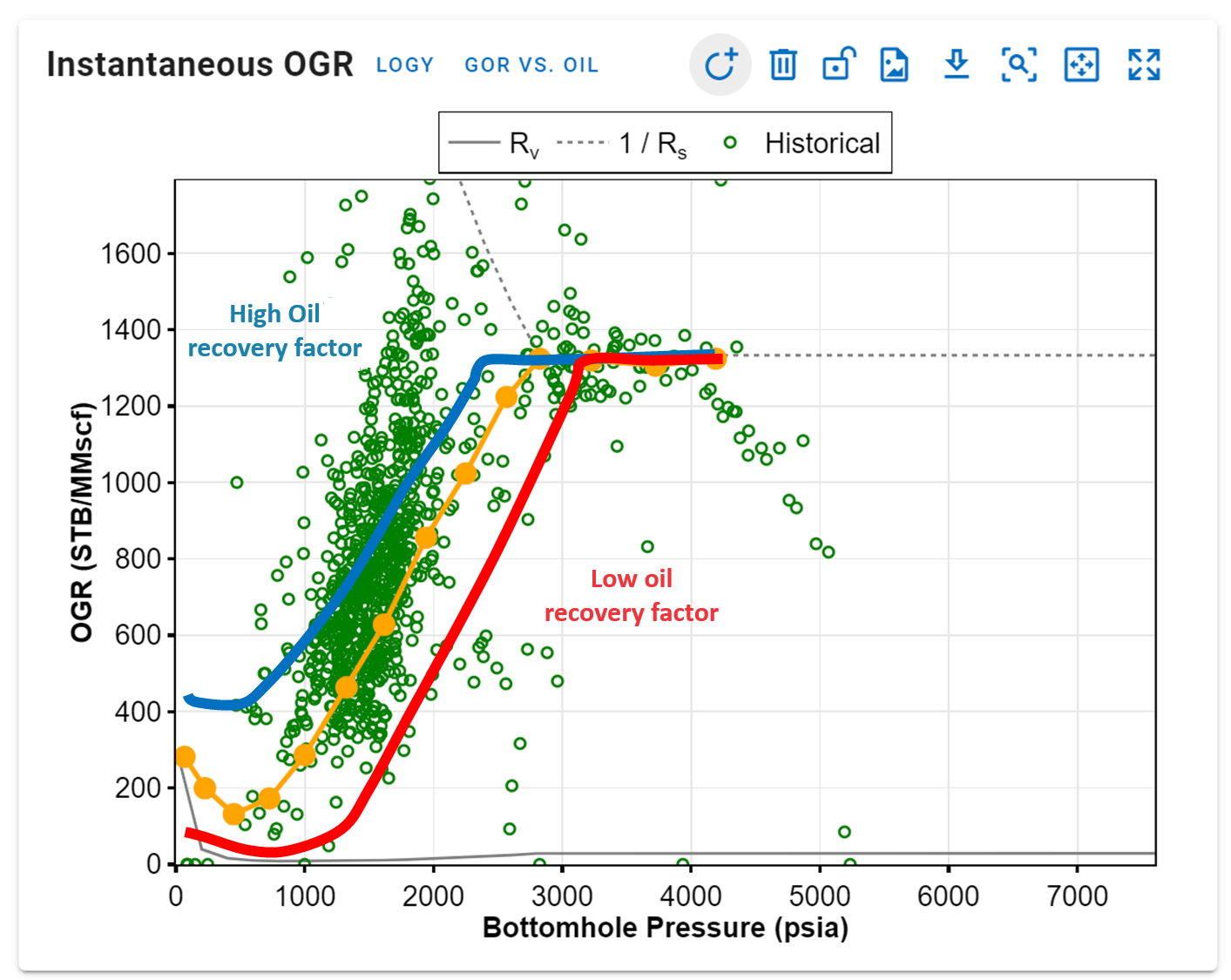
2.1. How should $ogr$ and $wgr$ be forecasted versus pressure?

$R_v$ and $1/R_s$ curves are generated from the EoS based on the PVT initialization. $R_v$, or solution oil-gas ratio, represents the minimum amount of oil expected to be recovered at the surface from gas production. It provides a lower bound for the expected oil-gas ratio when the oil phase becomes less mobile and gas remains the dominant flowing phase.

$1/R_s$, or the reciprocal of the solution gas-oil ratio, represents the maximum amount of oil that must be recovered to produce a unit volume of gas from solution. This provides an upper bound for the ratio forecast.

The forecasted ratio should remain within these physical bounds.

Above saturation pressure, $ogr$ data are typically close to the $1/R_s$ trend. The forecast should follow the historical data and then extrapolate reasonably to lower pressures, down to the abandonment pressure. $wgr$ typically decreases as pressure declines.

2.2. Reducing uncertainty in ratio forecasting - use analogs!

If yield or $gor$ is primarily controlled by flowing bottomhole pressure, the result may not vary significantly with the analog type, such as parent, edge, or fully bounded wells. In this case, the selected analog should have a similar producing history and sufficient production duration.

If yield or $gor$ is primarily controlled by average reservoir pressure, separate the analog wells by well type and select the trend that best matches the well being forecasted. Parent wells may show lower and flatter $gor$ behavior, while edge wells and fully bounded wells may show sharper increasing trends. The forecast should be bounded by the analog behavior, where fully bounded tight infill wells may represent the sharpest increase in $gor$, and parent wells may represent a lower bound for both magnitude and rate of change.

Finally, always use cumulative $GOR$ versus cumulative oil as a sanity check. A reasonable forecast should transition smoothly from the historical trend and generally show a realistic increasing trend without sudden jumps or discontinuities.

Impact of these forecasts on recovery factors

Oil EUR and oil recovery factor are usually most sensitive to the $OGR$ forecast. Gas EUR and gas recovery factor may be slightly more sensitive to the constructed $WGR$ forecast. In practice, the largest uncertainty is often associated with the oil-gas ratio forecast, which has the highest impact on calculated oil recovery.

3. Obtaining EURs from Recovery Factor Analysis

3.1. How can FMB methods be used to calculate EUR?

The FMB method estimates the contacted pore volume and the corresponding contacted hydrocarbons in place, such as $OOIP_{contacted}$ or $GIP_{contacted}$. To calculate EUR, the contacted hydrocarbons in place must be multiplied by the estimated recovery factor.

For example:

$$EUR_{oil}=OOIP_{contacted}\times RF_{oil}$$

3.2. How do we estimate a recovery factor?

The multiphase FMB method used in whitson⁺ does not require relative permeability inputs. Therefore, for forecasting purposes, whitson⁺ uses a recovery-factor workflow that also does not require relative permeability data. Instead, the producing ratios are forecasted directly. Although producing ratios are influenced by PVT behavior and relative permeability, forecasting the ratios directly allows recovery factor and EUR to be estimated without explicitly defining relative permeability curves.

3.3. Comparison of methods for calculating recovery factors

Recovery factors calculated from FMB Recovery Factor Analysis, numerical modeling, or simple material balance should be consistent when the producing-ratio forecast and abandonment pressure are consistent. In other words, if the producing $GOR$ at the end of history, the forecasted producing-ratio trend, and the abandonment pressure are the same, the calculated recovery factor should also be the same.

For unconventional reservoirs dominated by expansion-drive behavior, MFMB and numerical-model recovery factors should be consistent when the forecasted producing ratios and abandonment pressure are the same.

MFMB vs Numerical Model recovery factors

In MFMB, producing ratios are forecasted directly and then used with material-balance equations to calculate recovery factors and EUR. This is the opposite direction of a numerical simulation, where the model predicts producing ratios over time, which are then used to calculate recovery factors and EUR.

3.4. How to validate if the ratio forecast makes sense?

Plot cumulative $GOR$ versus cumulative oil. Check whether the forecasted points transition smoothly from the historical cumulative $GOR$ trend. If the forecast continues without sudden breaks, jumps, or unrealistic declines, the ratio forecast is likely reasonable. If a sudden discontinuity appears between the historical and forecasted points, the ratio forecast should be adjusted so that it aligns smoothly with the historical cumulative $GOR$ trend.

In cases where DCA EUR and MFMB EUR diverge, the $CGR$ vs pressure curve can be modified to achieve alignment, thereby adjusting the recovery factor for oil.

4. Relevant videos

4.1. New Multiphase Flowing Material Balance Method

4.2. How to interpret the multiphase FMB plot?

4.3. Linking Multiphase Flowing Material Balance method to Recovery Factor Calculations

Nomenclature

Variable	Definition	Units
$B_g$	Gas formation volume factor	RB/Mscf
$B_o$	Oil formation volume factor	RB/STB
$B_w$	Water formation volume factor	RB/STB
$b_M$	Multiphase productivity index	RB/day
$GIP$	Gas in place	Mscf
$G_p$	Cumulative produced gas	Mscf
$\dot{m}$	Mass flow rate	lbm/d
$M_g$	Cumulative mass of surface-produced gas	lbm
$M_o$	Cumulative mass of surface-produced oil	lbm
$M_T$	Total cumulative produced mass	lbm
$M_w$	Cumulative mass of surface-produced water	lbm
$MBT_M$	Mass material balance time	day
$N_p$	Cumulative produced oil	STB
$OGR$	Cumulative producing oil-gas ratio	STB/Mscf
$ogr$	Instantaneous producing oil-gas ratio	STB/Mscf
$OIP$	Oil in place	STB
$p$	Pressure	psia
$p_{wf}$	Flowing bottomhole pressure	psia
$q_g$	Gas production rate	Mscf/d
$q_o$	Oil production rate	STB/d
$q_w$	Water production rate	STB/d
$R_s$	Solution gas-oil ratio	Mscf/STB
$R_v$	Solution oil-gas ratio	STB/Mscf
$RF_g$	Gas recovery factor	-
$RF_o$	Oil recovery factor	-
$S_g$	Gas saturation	-
$S_o$	Oil saturation	-
$S_w$	Water saturation	-
$t$	Time	day
$V_p$	Contacted reservoir pore volume	RB
$WGR$	Cumulative producing water-gas ratio	STB/Mscf
$wgr$	Instantaneous producing water-gas ratio	STB/Mscf
$W_p$	Cumulative produced water	STB
$\beta$	Mixture density	lbm/RB
$\rho$	Density	lbm/ft³
$\rho_{o,sc}$	Oil density at standard conditions	lbm/ft³
$\rho_{g,sc}$	Gas density at standard conditions	lbm/ft³
$\rho_{w,sc}$	Water density at standard conditions	lbm/ft³
$\zeta_g$	Component concentration of gas	Mscf/RB
$\zeta_o$	Component concentration of oil	STB/RB
$\zeta_w$	Component concentration of water	STB/RB