Gas Flowing Material Balance
This methodology should only be used for dry/wet gas wells.
1. Theory
This module is designed based on the work presented by Palacio and Blasingame (1993) known as "Conventional Gas Flowing Material Balance". The method involves plotting the rate-normalized pseudopressure \(\left(\frac{\Delta p_p}{q_g}\right)\) vs. material balance pseudotime (\(t_{ma}\)). During pseudosteady-state flow, this results in a straight line with slope inversely proportional to the contacted pore volume \(\left(V_p\right)\).
Conventional gas FMB is given by:
Where \(\Delta p_{p}\) is real gas pseudo-pressure drop defined as:
where the subscripts \(i\) and \(wf\) reflect initial and well flowing bottomhole condition, respectively. Gas viscosity (cp) is represented by \(\mu_g\), while Z is gas compressibility factor and \(p\) is pressure (psia).
Palacio and Blasingame (1993) introduced material balance pseudotime, \(t_{ma}\) (days) to account for changes in gas viscosity and compressibility as the average reservoir pressure declines.
Where \(\bar{p}\) denotes the average reservoir pressure in psia, \(q_g\) is gas production rate in Mcf/d and \(c_t\) is total compressibility in 1/psi.
Total compressibility accounts for the compressibility of the fluid phases present in the system as well as the rock compressibility, and is given by
where \(c_g\), \(c_o\), \(c_w\), and \(c_r\) denote gas, oil, water and formation (rock) compressibility, respectively. The default value of \(c_r\) is 4x10\(^{-6}\) 1/psi and \(c_w\) is 2.8x10\(^{-6}\) 1/psi in whitson+.
According to Eq. \eqref{eq:gas-FMB}, the slope of the straight line during pseudo-steady-state flow is denoted by \(m_{pss}\) in psia\(^2\)/cp-Mscf,
Original gas in place is calculated by,
with gas formation volume factor given by,
Rearranging Eq. \eqref{eq:slope-of-straight-line} with Eqs. \eqref{eq:OGIP} and \eqref{eq:Bg}, then contacted pore volume \(\left(V_p\right)\) in Mscf can be determined.
Subscript \(sc\) refers to standard condition and \(T\) is temperature in Rankine.
From simple material balance (ignoring rock and water compressibility),
Please note that this method requires the user to input first guess of \(G_i\) to determine \(t_{ma}\). It uses an iterative procedure to correctly estimate the \(G_i\).
2. Workflow
Gas FMB Workflow
- Using the provided PVT data, calculate initial properties (\(B_{gi}\), \(c_{gi}\), \(\mu_{gi}\) and \(m(p_{i})\)).
- From the production data, calculate the following properties for every time step:
- Cumulative gas production (\(G_p(t)\))
- Using an initial guess of the gas in place (\(G_{i-guess}\)), calculate average gas formation volume factor (\(\bar{B_g}(t)\)) using Eq. \eqref{eq:Average-Bg}
- From the PVT data, determine the average pressure (\(\bar{p}(t)\)) that gives \(\bar{B_g}(t)\)
- Similarly, interpolate for average gas viscosity and compressibility (\(\bar{\mu_g}(t)\) and \(\bar{c}(t)\)) at \(\bar{p}(t)\)
- Material balance pseudo time using Eq. \eqref{eq:MB-Pseudotime}
- From PVT data, calculate \((p_{p_{wf}})\)
- Rate-normalized pseudopressure \(\left(\frac{\Delta p_{p}(t)}{q_g(t)}=\frac{p_{p_{i}}-p_{p_{wf}}}{q_g(t)}\right)\)
- Plot material balance pseudotime \(\left(t_{ma}\right)\) on the x-axis and rate-normalized pseudopressure \(\left(\frac{\Delta p_{p}(t)}{q_g(t)}\right)\) on the y-axis.
- Find slope (\(m_{pss}\)) and intercept (\(b_{pss}\)).
- Calculate contacted pore volume (\(V_p\)) using Eq. \eqref{eq:pore-volume}.
- Calculate original gas in place (\(G_i\)) using Eq. \eqref{eq:OGIP}.
3. Gas Flowing Material Balance (FMB) accounting for Rock Compressibility
Consider a tank with initial volume \(V_{pi}\) containing gas at initial pressure \(p_{i}\) and water at initial saturation \(S_{wi}\). The compressibility of the tank (rock) and water are \(c_r (p)\) and \(c_w (p)\). Water is assumed to be immobile in the system. If water is mobile, the multiphase FMB method should be used instead. If the initial volume of gas in place is \(G_{i}\), then we can express this in terms of the tank volume as
After removal of a certain volume of gas (\(G_p\)) the tank pressure falls to p, the insitu volume of gas is given by
where (\(Υ_V\)) and (\(Υ_w\)) are the rock and water volume multipliers, respectively. We assume that (\(Υ_w (p)\)) is 1 in this module and that water compressibility, \(c_w\), is 2.8x10\(^{-6}\) 1/psia.
Substituting for \(V_{pi}\) from Eq. \eqref{eq:GiBgdi}, we have
or
4. Computing Original Gas in Place with Adsorption
Shale reservoirs possess a remarkable capacity to store methane through a process known as "adsorption." This involves gas molecules adhering to the organic material within the shale, creating a near-liquid state of condensed gas. A useful analogy is to envision a magnet sticking to a metal surface or lint clinging to a sweater, illustrating the concept of adsorption versus absorption, where one substance is trapped inside another like a sponge soaking up water. The adsorption process is reversible due to its reliance on weak attraction forces.
Compared to conventional reservoirs, shale reservoirs can store significantly more gas in the adsorbed state, even when compression is applied at pressures below 1000 psia. Notably, the gas stored in shale is predominantly held in the adsorbed state, as opposed to being free gas. This is because the volume of the cleat or fracture system within shale is relatively small compared to the overall reservoir volume. As a result, the pressure volume relationship is commonly described through the desorption isotherm alone.
Langmuir Isotherm
The release of adsorbed gas is commonly described by a pressure relationship called the Langmuir isotherm. The Langmuir adsorption isotherm assumes that the gas attaches to the surface of the shale, and covers the surface as a single layer of gas (a monolayer). At low pressures, this dense state allows greater volumes to be stored by sorption than is possible by compression.
The typical formulation of the Langmuir isotherm is:
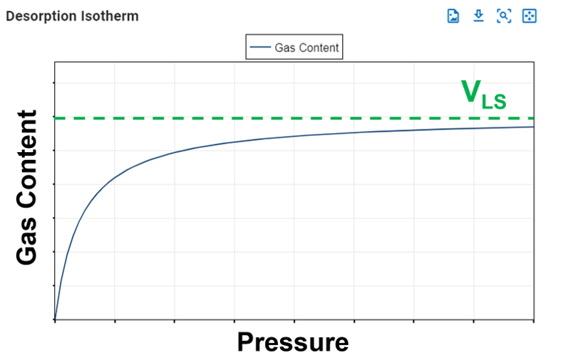
Langmuir Volume, VLS
The Langmuir volume is the maximum amount of gas that can be adsorbed by a shale at an "infinite pressure". The plot below of a Langmuir isotherm demonstrates that gas content asymptotically approaches the Langmuir volume as pressure increases to infinity.
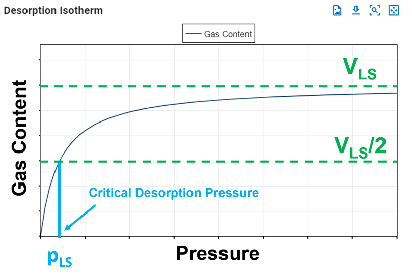
Langmuir Pressure, pLS
The Langmuir pressure, or critical desorption pressure, is the pressure at which one half of the Langmuir volume can be adsorbed. As seen in the figure below, it changes the curvature of the line and thus affects the shape of the isotherm.
Computing Original Gas in Place (OGIP)
Ambrose et al.[1] argue that the free OGIP must be corrected for the adsorbed gas that occupies some of the hydrocarbon pore volume (HCPV). If porosity is estimated from core plugs where core preparation has removed the adsorbed gas, then the OGIP will be overestimated.
The convention of reporting OGIP when adsorption is included, is to report it in units of scf/ton (standard cubic feet per short ton). For a fluid system having only dry/wet gas and water, the total OGIP is
where
and with \(C_1\approx 5.7060\) and \(C_2\approx1.318\cdot10^{-6}\) are unit conversion factors. The shale saturation is capped at \(1-S_{wi}\), meaning the maximum amount of shale you can have is the entire HCPV. Hence, this will make the results independent of the adsorption numbers when violating this constraint.
The OGIP resolved in the ARTA and GFMB features yields the free OGIP. We can use this volume to compute the rock mass, which in turn can be used to calculate the adsorbed OGIP. Multiplying equation \eqref{eq:freegasperton} with the rock mass (\(G=\hat{G}_f m_r\)) gives the free OGIP in units of scf. Solving for the rock mass yields
This rock mass can then be multiplied by equation \eqref{eq:adsorbedgasperton} to get the adsorbed OGIP in scf, i.e.,
Total Compressibility when Adsorption is ON
In order to honor mass balance, it becomes necessary to modify total system compressibility when accounting for adsorption. Total system compressibility can be determined using the following equation:
The derivation of this equation is shown here and is constructed upon Ambrose et al.[1].
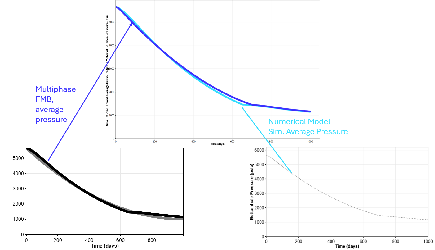
5. Simulation vs. FMB Average Pressure
There is an important distinction between the average reservoir pressure calculated from a numerical simulation model and the material balance pressure back-calculated by FMB.
The simulation-derived average pressure is calculated from the pressure distribution across the grid cells using the averaging or weighting method defined by the simulator, such as pore-volume or hydrocarbon-pore-volume weighting.
In contrast, the FMB average pressure represents the equivalent pressure of a single, well-mixed tank containing the same total fluid mass. It is obtained from the material balance relationship and accounts for pressure-dependent fluid properties and compressibility, including the gas behavior.
The two pressure estimates are equal only when the reservoir behaves as a sufficiently uniform tank with negligible pressure and composition gradients. In real reservoirs, pressure depletion, multiphase behavior, and compositional variation can cause the two values to differ. These differences may become particularly noticeable during transient flow, pressure buildup, or shut-in periods.