Equation of State Model
1. Introduction
An equation of state (EOS) model is a functional relationship that relates pressure-volume-temperature-composition (PVTx). There are various EOS models that can describe petroleum systems, but the most commom industrial models are cubic EOS models. A cubic EOS model is a model that can be described as a cubic polynomial with respect to molar volume (\(v\)) or Z-factor. The most commonly used cubic EOS models are the 1979 Peng-Robinson (PR) model, and Soave's modification to the Redlich-Kwong (SRK) model.
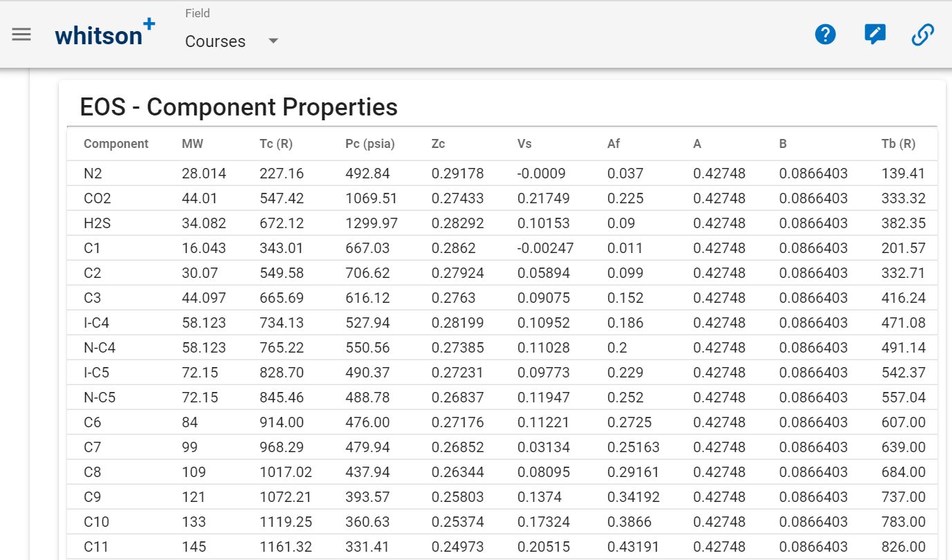
A cubic EOS model is made up of two parts: (a) the component properties (\(T_c\), \(p_c\), \(\omega\), etc.) and (b) the binary interaction parameters (BIPs). The component properties are used to describe the individual components phase behavior, like the vapor pressure. Component properties for known isomers (e.g. non-hydrocarbons like \(\mathrm{N}_2\) or hydrocarbons like methane) are typically pre-defined as library values. However, it is important to note that different software use different library component values that can and will have an impact on the mixture phase behavior predictions.
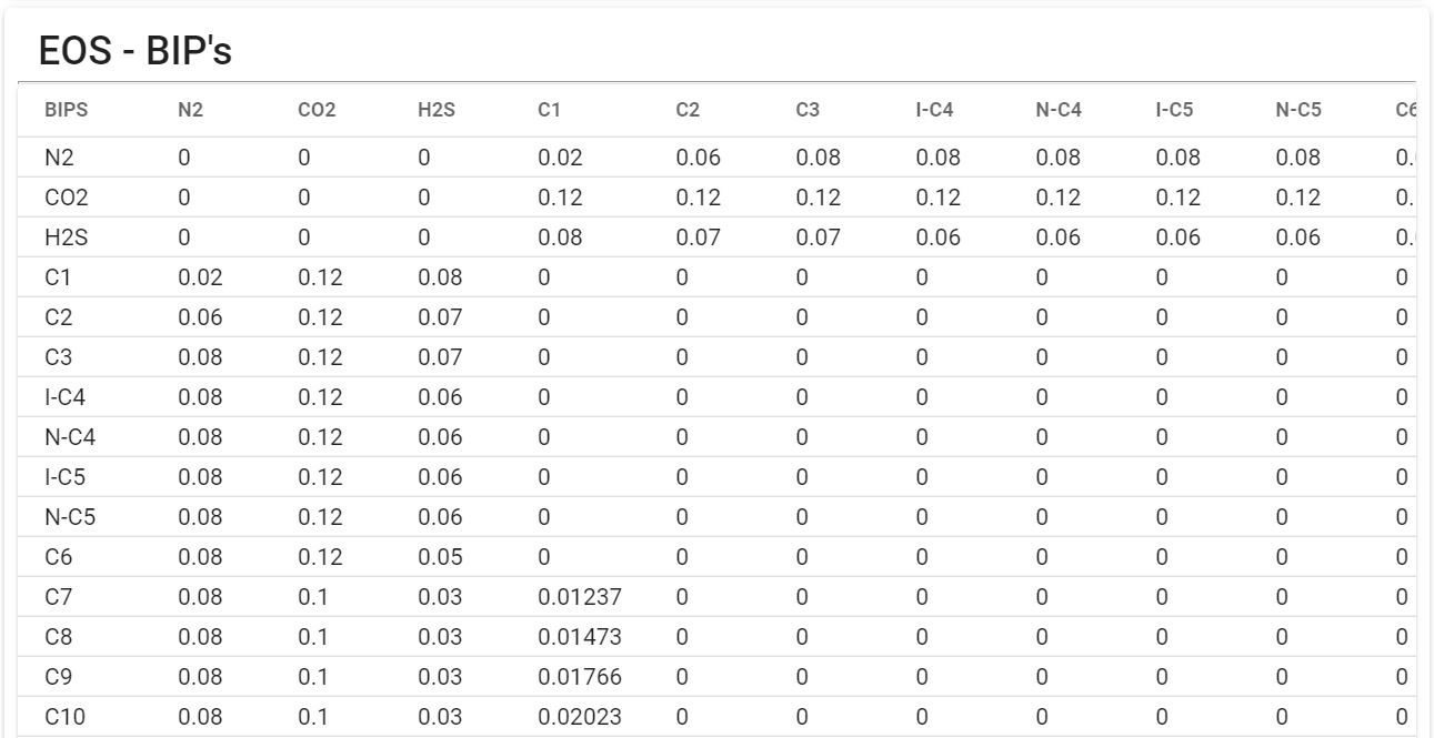
The second set of values are the BIPs, which are correction terms to the averaging-rules / mixing-rules used to go from a mixture of \(N_c\) components to a single mixture component. There is a single BIP between each component, and is therefore often shown as an \(N_c \times N_c\) square matrix. The BIPs matrix is symetric (\(k_{ij}=k_{ji}\)) because the BIP between component \(i\) and \(j\) is the same as the BIP between component \(j\) and \(i\). The BIP between a component and itself (i.e. \(k_{ii}\)) is set to zero and therefore the diagonal of the BIP matrix is zero. BIPs typically range from -0.1 to 0.2 and have a tendency to increase with increasing difference in molecular weight (for example the BIP between \(\mathrm{C_1}\) and \(\mathrm{C_2}\) is less than the BIP between \(\mathrm{C_1}\) and \(\mathrm{C_{36+}}\)). There is no physical reason why the BIPs should not be negative, but as a note of caution one should always quality control the EOS model if BIP tuning is applied because unconstrained tuning can easily lead to non-physical phase behavior predictions (crossing K-values or three-phase behavior).
One of the main challenges of EOS model development is to estimate the component properties and BIPs for the \(\mathrm{C_{7+}}\) fraction. This is what is called \(\mathrm{C_{7+}}\) characterization or plus charaterization. There are multiple correlations for estimating the critical properties using the molecular weight, specific gravity (density), and the normal boiling point. However, there is sometimes need for some additional tuning to these properties to get a good fit to the measured PVT data. To get the BIPs, there is typically a set of library values for the non-hydrocarbon to hydrocarbon BIPs, while the hydrocarbon-hydrocarbon pairs are either set to zero, or tuned to fit the PVT data. One approach is to tune the BIPs by using a correlation like the Chueh-Prausnitz model. Explicit tuning (often between the lightest and heaviest fraction) may also be needed to adequately fit the PVT data.
Useful links for additional reading
For an introduction to EOS models and EOS modeling, please read this article or navigate to the whitson wiki on the EOS model section. For a great article on EOS model transfer between different software, please read this article, or if you are interested in learning more about using ASTM D2892 data for \(\mathrm{C}_{7+}\) characterization you should read this article. There is also a great article on EOS model lumping here. Or perhaps you need to quality control your EOS model, then you can read up on this here.
2. EOS Models in whitson+
A single or multiple EOS models can be defined for a given field/basin in whitson+. A field should have at least one EOS model to do any calculations in whitson+. For any given field, the list of existing EOS models can be accessed with the EOS Model button in the navigation menu of whitson+ as shown in figure below
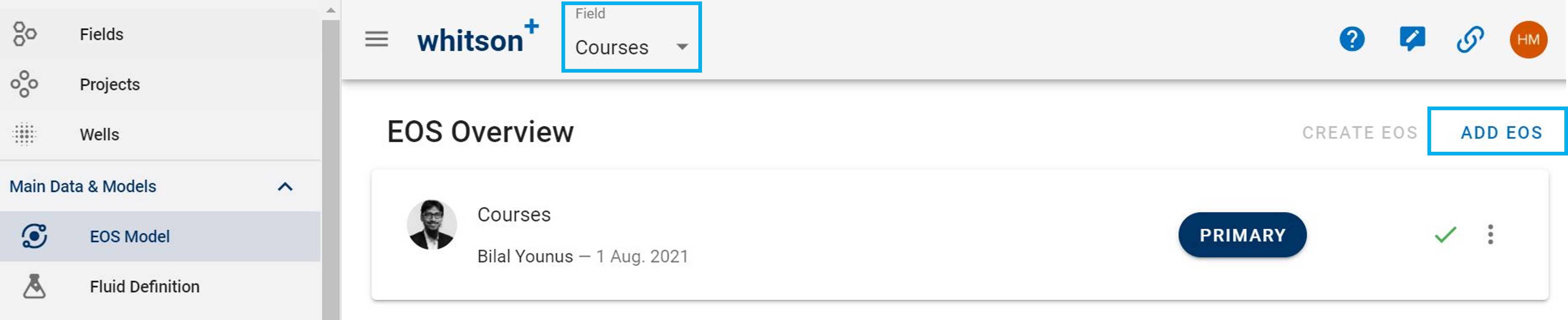
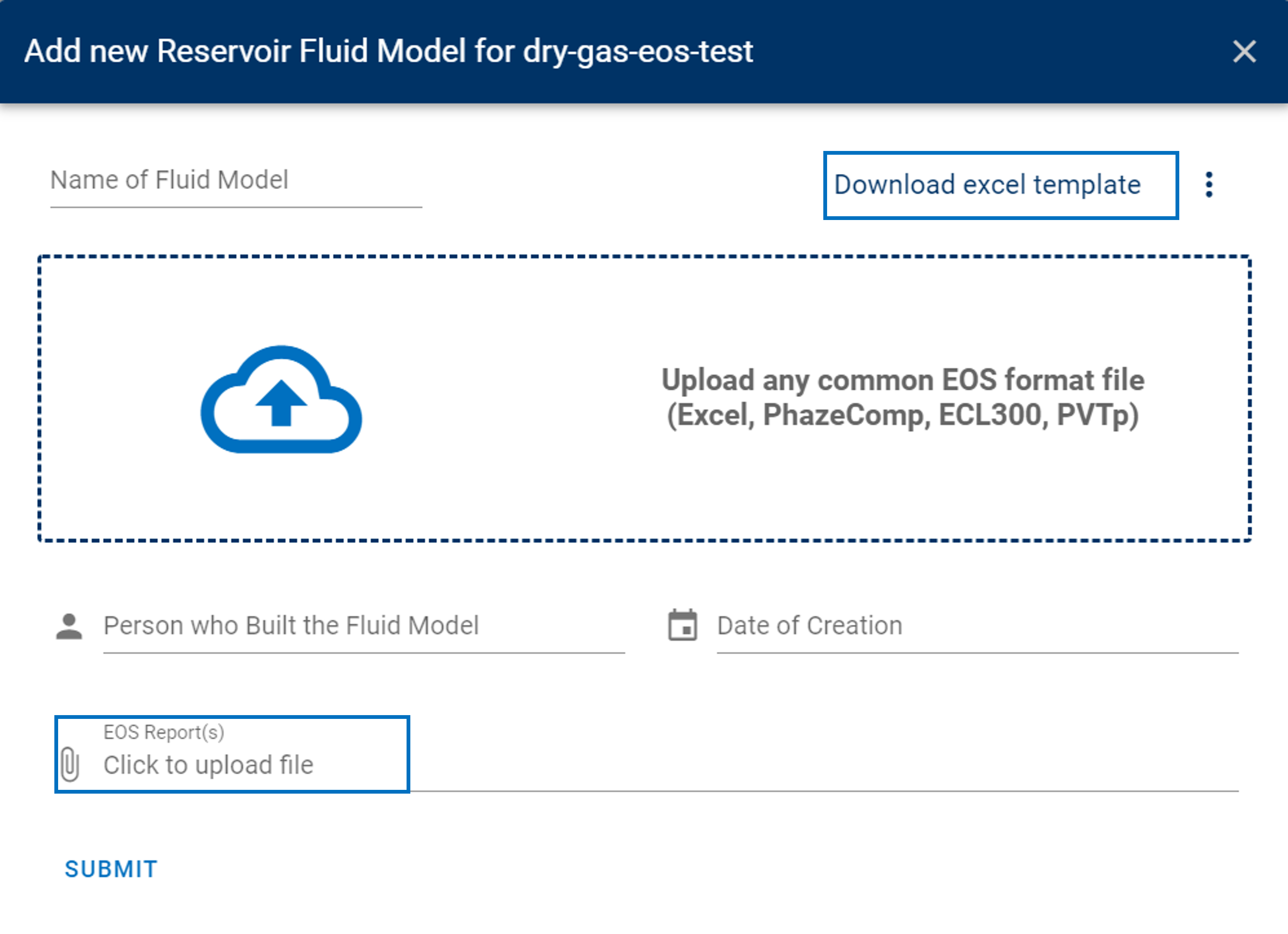
Multiple EOS models can be added for a given field using Add EOS button shown in figure above. When adding a new EOS model, it is important that the EOS model name should not contain any blank spaces. The model can be added in various formats as shown in figure below. The Excel template for uploading the EOS model can be downloaded using the highlighted option in figure below. Also, any documentation regarding the EOS model can be uploaded as shown below.
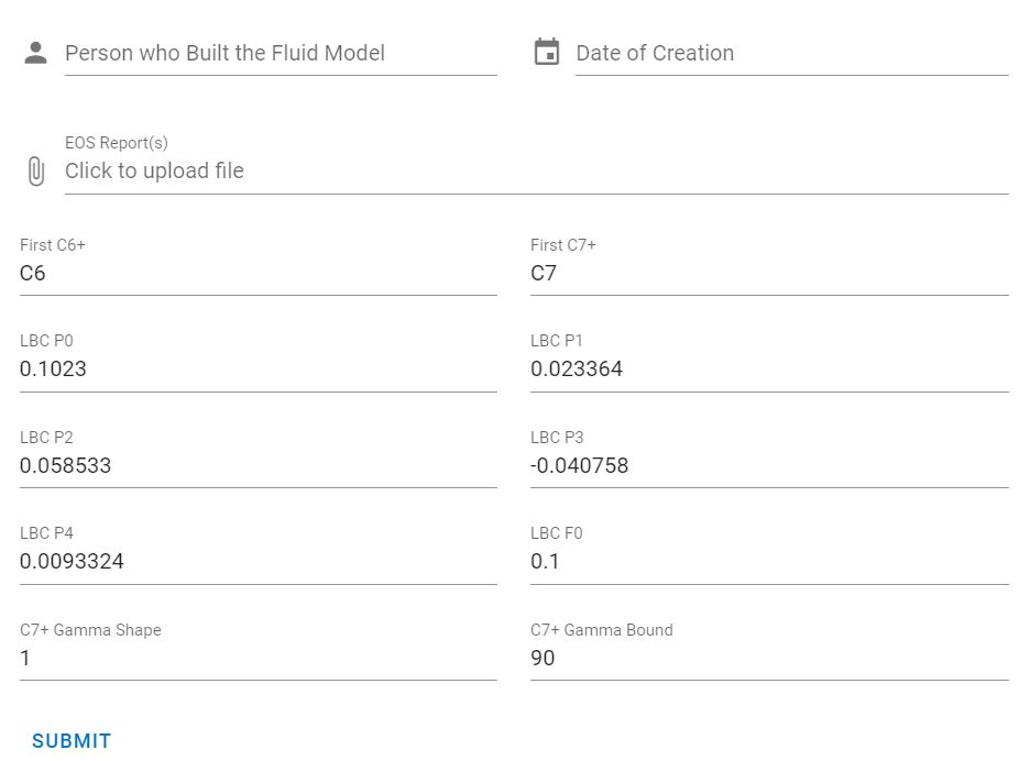
If options other than Excel template are used to upload the EOS model, some additional information will need to be provided by the user as shown in the figure below. The values are filled in with default values and should be replaced by the user with the tuned/representative values for the field and the EOS model, where applicable. First \(\mathrm{C_{6+}}\) means the first component in the EOS model that contains components associated to single carbon number \(\mathrm{C_{6}}\) fraction and same goes for First \(\mathrm{C_{7+}}\).
In the presence of the multiple EOS models for a given field, a primary EOS model should be selected that is used in all calculations. This can be done by clicking on the menu option of the specific EOS model as shown in figure below and click on Make primary fluid model . Any EOS model used in whitson+ for calculations require a seed feed table, which can be uploaded using the option Upload seed feeds in the figure below.
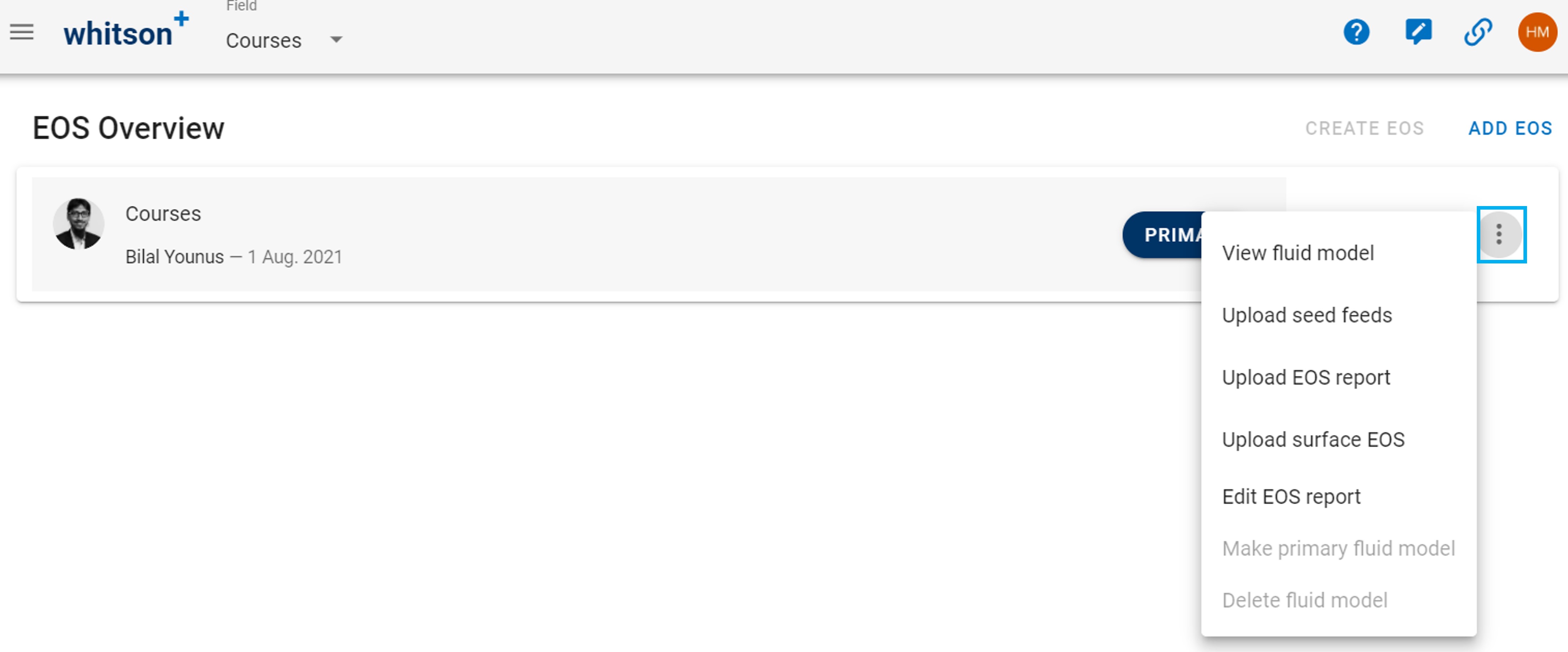
Sometimes, accurate EOS calculations require two different EOS models such that one for calculations at reservoir conditions (reservoir EOS) and one for calculations at surface conditions (surface EOS). Any EOS model uploaded to whitson+ is considered as Reservoir EOS. A separate Surface EOS (if available) can be appended to a Reservoir EOS using the option Upload surface EOS as shown in the figure above.
The EOS model parameters can be seen by clicking on the option View fluid model as shown in the figure above. Important information about the model appears as shown in figure below.
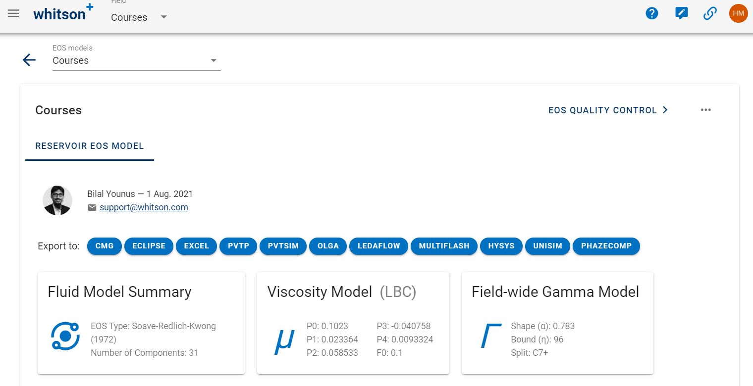
The information includes:
- Name of the person who built the EOS model and the date (i.e. when the model was built)
- Model summary information e.g. the type of EOS and the number of components
- Tuned parameters of the LBC viscosity model
- Gamma molar distribution model parameters applicable to the field/basin
Moreover, the EOS model can be exported into many third-party formats with a click of a buttion as shown in figure above. Another important feature that can be accessed is EOS Quality Control as shown in figure above. By clicking on this button, a very comprehensive set of quality checks are done on the selected EOS model and the results are shown. Read this article to know more about the EOS quality control methods. When the EOS model is selected for viewing, the component properties table and binary interaction parameters table also appear as shown in the figures below
2.1. whitson+ Default EOS Model
As mentioned earlier, an EOS model is a pre-requisite for doing any calculations in whitson+. If an EOS model is not available for a specific field or basin, it is possible to use a default EOS model available in whitson+ for doing approximate calculations. The model can be accessed as shown below.
It is very important to note that this EOS model is NOT tuned to any PVT data and the calculated results should not be trusted with high confidence. The EOS model is based on properties of \(\mathrm{C_{7+}}\) fractions from the PVT Package default correlations. The intention with this EOS model is to provide the user some means to do relevant phase behavior calculations for a specific field in whitson+, only when a tuned EOS model is not available. We highly recommend tuning an EOS model to measured PVT data (when available), and use the tuned EOS model for calculations instead.
It is also important to mention here that the seed feed table associated to this EOS model contains zero mole fractions of non-hydrocarbons. Therefore, the user should specify the known/measured amounts of non-hydrocarbons when generating wellstream composition in whitson+ using one of the available methods.
2.1.1. Default EOS Assumptions and Limitations
The default Equation of State (EOS) is based on a predefined set of representative fluid systems and is intended to provide a generalized starting point for modeling. As a result, cases that fall beyond the bounds of this predefined fluid range may not be fully captured by the default EOS behavior.
In addition, the default EOS uses an untuned viscosity model. Since viscosity behavior can vary significantly across different reservoirs and fluid systems, viscosity predictions generated using the default EOS may not be representative of field-specific conditions. For improved accuracy, it is recommended to tune the EOS and viscosity model using available field-specific PVT data.
2.2. whitson+ Dry or Wet Gas EOS Model
For fields/basins producing dry or wet gas fluids, whitson+ dry/wet gas EOS model can be used to describe the phase behavior if an EOS model does not exist for the given field. The model can be accessed the same way as default EOS model as described above.
The model is built using comprehensive set of dry/wet gas sample compositions. The methane content varies in the available PVT samples from 70 mol% to 90 mol% and \(\mathrm{C_{6+}}\) varies from 0.3 mol% to 2 mol%. Calculated PVT data (gas Z-factors and viscosities) at different temperatures varying from 60 °F to 260 °F were used to validate the EOS model. It is important to mention that \(\mathrm{N_{2}}\) and \(\mathrm{CO_{2}}\) contents in the available PVT samples were less than 2 mol% and \(\mathrm{H_{2}S}\) was zero mol%. The EOS model may not be as accurate as it should be for samples with large amounts of non-hydrocarbons.
3. Important Notes Regarding EOS Export/Import
It is recommended to read this article, which higlights most of the issues in transfering the EOS model from one package to another and discusses the important calculations required to make sure if the EOS is correctly imported.
3.1. HYSYS
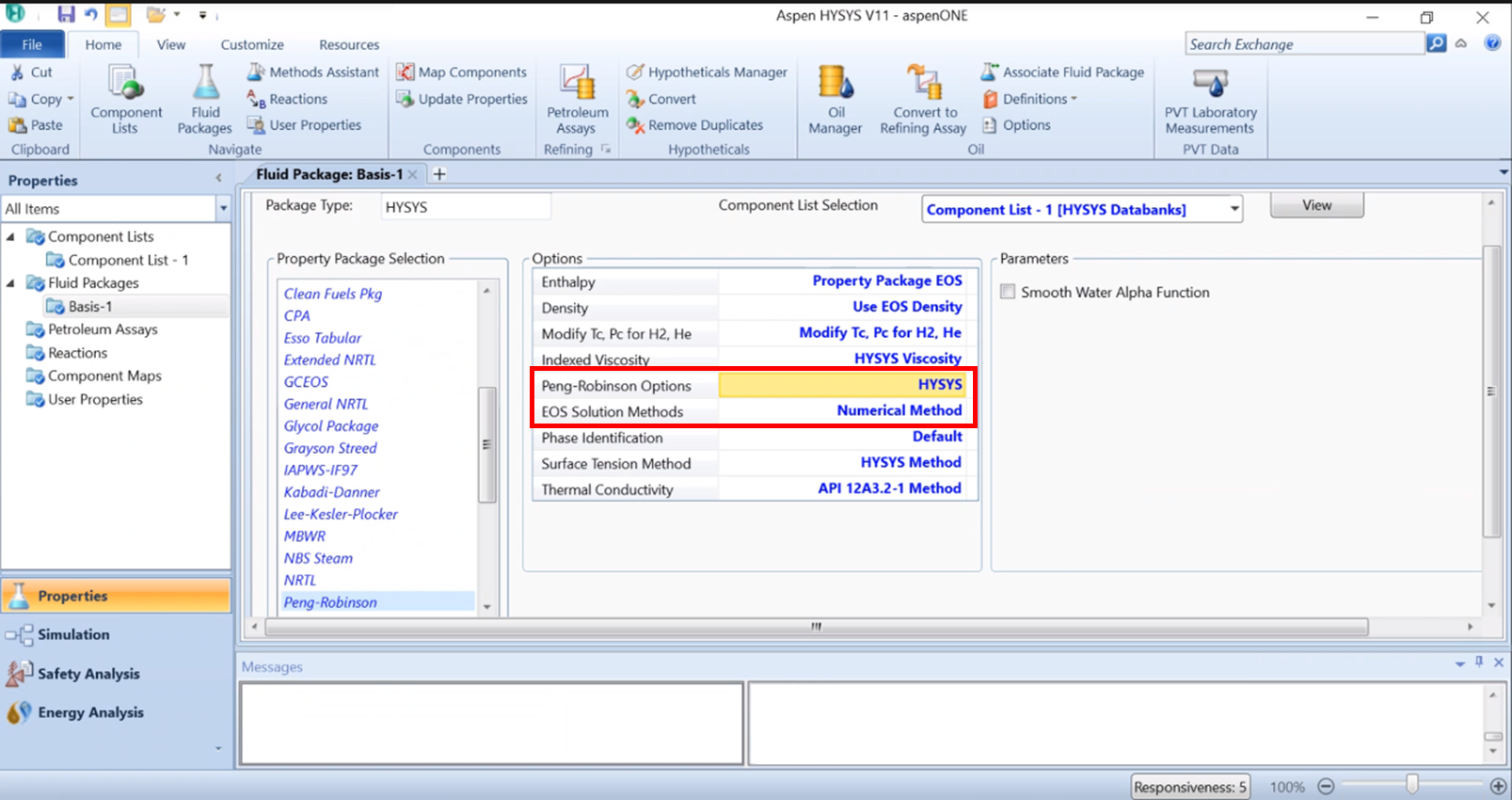
When importing an EOS model into HYSYS, make sure to:
- Select "HYSYS" under Peng-Robinson Options
- Choose "Numerical Method" under EOS Solution Methods
Warning
HYSYS does not allow the EOS coefficients \(\Omega_a\) and \(\Omega_b\) to be changed. Tuning those EOS coefficients is not common practice and not something we recommend doing in general, as it can lead to physical and thermodynamical inconsistencies. For more information, please contact us at support@whitson.com.
3.2. PVTp
-
Use the Import Feature and import Eclipse300 file
-
Change the vc column with the critical viscosities for the LBC correlation (VcVis)
-
IMPORTANT: Check that all properties are imported correctly, for example:
- Component Tb and SG — most times replaced by PVTp internal values
- Heavier component properties — most times are not correctly imported
- LBC coefficients — may not be imported correctly
3.3. PVTsim
The “Import from Eclipse” only works if you have a composition associated with the EOS.