Fractional RTA

1. Theory

There have been many studies showing that infinite acting, linear flow is the dominant flow regime in multifractured horizontal wells for tight unconventional reservoirs. The most common production analysis of linear flow was first introduced by Wattenbarger et al. in 1998. They proposed analytical solutions for both constant rate and constant pressure. In reality, rates and pressures change simultaneously. To account for that, the principle of superposition is applied.

In 1993, Palacio and Blasingame introduced the concept of material balance time (MBT). Material balance time

• is a superposition time function.
• converts variable rate data into an equivalent constant rate solution.
• is rigorous for a boundary-dominated flow regime.
• works well for transient data, but is only an approximation (errors can be up to 20% for linear flow).

In the whitson⁺ classical RTA module, material balance time is the default time function. Therefore, the theory for the constant rate solution is emphasized in this part of the manual. On the other hand, there is an option to use the constant pressure solution by selecting "Real Time" as a function of time, as presented here.

The purpose of conducting this analysis is to determine the linear flow parameters (LFP=$A\sqrt{k}$) and drainage volume by interpreting production data. Using Arps' equation with respect to the end-of-linear-flow time $(t_{elf})$, a production forecast can be made.

1.1. Assumptions

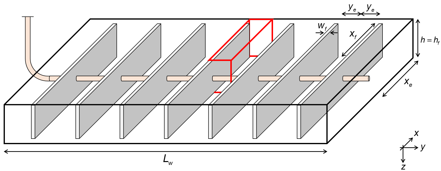
Fig. 1: Wellbox model

Fig. 1 shows the geometry of the well used as a base assumption of these analyses. The fracture is assumed to have infinite fracture conductivity, such that the linear flow is perpendicular to the fracture. Additionally, this module assumes single-phase flow with no flow beyond the fracture tip (\(x_e=x_f\) and \(h=h_f\)), i.e. a fully-penetrating fracture (1D model).

1.2. Superposition Time

There are two superposition time function options in whitson⁺: material balance time and linear superposition time. In addition, real time can be used (called "Variable Pressure" in other tools), where no superposition time function is applied.

1.2.1. Material Balance Time (Default in Software)

The use of material balance time is common in rate-transient analysis, and it is the default in whitson⁺. Mathematically, material balance time, MBT \((t_c)\), is expressed as: $$\begin{equation} \label{MBT} t_c=\frac{Q(t)}{q(t)} \end{equation}$$

where \(Q(t)\) and \(q(t)\) are cumulative production and production rate at time \(t\).

1.2.2. Linear Superposition Time

Mathematically, linear superposition time $(t_{\text{linear}})$ is expressed as:

$$\begin{equation} \label{linear_superposition_time} t_{\text{linear}} = \left( \sum_{j=1}^{n} \frac{q_j - q_{j-1}}{q_n} \cdot \sqrt{t_n - t_{j-1}} \right)^2 \end{equation}$$

1.2.3. Linear Superposition Corrected Pseudotime

Mathematically, linear superposition corrected pseudotime \((t_{\text{ca,linear}})\) is expressed as:

$$\begin{equation} \label{linear_superposition_corrected_pseudotime} t_{\text{ca,linear}} = \left( \sum_{j=1}^{n} \frac{q_j - q_{j-1}}{q_n} \cdot \sqrt{t_{ca,n} - t_{ca,j-1}} \right)^2 \end{equation}$$

where \(t_{\text{ca}}\) denotes the corrected pseudotime evaluated at each rate change. In this formulation, real time in the linear superposition function is replaced by corrected pseudotime so that pressure-dependent changes in gas viscosity and total compressibility are accounted for during variable-rate gas flow.

1.3. Phase

You can choose to run the classical RTA analysis with one of the following rates:

• Oil (Surface)
• Gas (Surface)
• Water (Surface)
• Hydrocarbon (Reservoir)
• Liquid (Reservoir)
• Total (Reservoir)
• Oil Pseudopressure

Hydrocarbon reservoir rates are calculated from surface rates using PVT and bottomhole pressures as follows

$$\begin{equation} \label{eq:hc_rate} q_{hc} = q_{o,res} + q_{g,res} \end{equation}$$

Liquid reservoir rates are calculated from surface rates using PVT and bottomhole pressures as follows

$$\begin{equation} \label{eq:liq_rate} q_{liq} = q_{o,res} + q_{w,res} \end{equation}$$

Total reservoir rates are calculated from surface rates using PVT and bottomhole pressures as follows

$$\begin{equation} \label{eq:tot_rate} q_{tot} = q_{o,res} + q_{g,res} + q_{w,res} \end{equation}$$

In which $q_{o,res}$, $q_{g,res}$, and $q_{w,res}$ can be calculated as follows

$$\begin{equation} \label{eq:res_gas} q_{g,res} = \frac{q_g-R_sq_o}{1-R_sr_s}B_{gd} \end{equation}$$

$$\begin{equation} \label{eq:res_oil} q_{o,res} = (q_o-\frac{q_{g,res}}{B_{gd}/r_s})B_o \end{equation}$$

$$\begin{equation} \label{eq:res_water} q_{w,res} = q_wB_w \end{equation}$$

The PVT properties solution GOR, $R_{s}$, oil formation volume factor, $B_{o}$, solution CGR, $r_{s}$, gas formation volume factor, $B_{gd}$, and water formation volume factor, $B_{w}$ are all evaluated at the flowing bottomhole pressure, $p_{wf}$, every day to calculate total rates.

If gas (surface) is used for liquid-rich systems (oil rate, $q_{o,sc}$, greater than 0), the oil rate is added as an equivalent gas volume using this formula:

$$\begin{equation} \label{eq:wet_gas_rate} q_{g,wet} = q_{g,sc} + q_{o,sc}C_{og} \end{equation}$$

where \(C_{og}\) is a conversion from surface-oil volume in STB to an "equivalent" surface gas in scf:

$$\begin{equation} \label{eq:cog} C_{og} = 133,000 \frac{\gamma_{og}}{M_{og}} [scf/STB] \end{equation}$$

The $M_{og}$ is estimated using the Cragoe correlation.

$$\begin{equation} \label{eq:cragoe} M_{og} = \frac{6,084}{\gamma_{api}-5.9} \end{equation}$$

This rate, \(q_{g,wet}\), is typically referred to as a "wet" or "fat" gas rate.

1.4. Oil Pseudopressure

Traditionally, analytical solutions developed for oil wells assume that oil PVT properties exhibit only weak pressure dependence. Under this assumption, oil viscosity and oil formation volume factor are treated as constant. This simplification is generally reasonable for slightly compressible liquids over limited pressure ranges; consequently, most classical analytical solutions for oil reservoirs are formulated directly in terms of pressure.

In reality, however, oil PVT properties are not strictly constant. Above the bubble-point pressure, oil viscosity increases with increasing pressure, while oil formation volume factor decreases. Of greater importance is the variation of the combined term $B_o$ $μ_o$, which directly appears in governing flow equations. Neglecting pressure dependence in this term can introduce systematic bias into estimates of permeability, skin, and well productivity, particularly under conditions of large pressure drawdown. Failure to account for pressure-dependent PVT behavior can lead to errors in the characterization of reservoir and fracture properties.

In low-permeability and unconventional reservoirs, geomechanical effects further complicate the flow response. Changes in effective stress associated with pressure depletion can lead to pressure-dependent permeability, commonly represented by an exponential relationship of the form

$$\begin{equation} \label{eq:oilpseudo} k_{m}(p) = exp[\gamma_r(p-p_i)] \end{equation}$$

where $\gamma_r$ is a rock stress-sensitivity parameter. Incorporating pressure-dependent permeability directly into the flow formulation ensures that both fluid property variations and geomechanical effects are consistently captured during analysis.

To account for pressure-dependent oil properties in a manner analogous to gas-well analysis, the concept of oil pseudopressure is introduced. Oil pseudopressure reformulates the governing flow equation by embedding the pressure dependence of oil viscosity, oil formation volume factor, and permeability into an integral transform. In its general form, oil pseudopressure is defined as:

$$\begin{equation} \label{eq:oilpseudo1} p_{po}(p) = B_{oi}\mu_{oi}= \int_{p_{ref}}^{p_i} \frac {k_m (p)}{B_o(p) \mu_{o} (p)} dp \end{equation}$$

where $p_i$ is the initial reservoir pressure and $𝑝_{𝑟𝑒𝑓}$ is a reference pressure.

Oil pseudopressure properly accounts for pressure-dependent oil PVT property variations under undersaturated conditions, where the flowing bottom-hole pressure remains above the bubble-point pressure, gas remains in solution, and multiphase flow is absent.

1.5. Rate Normalized Pressure (RNP)

Rate Normalized Pressure (RNP) is useful for production analysis where flowing pressures and rates change through time. It is defined as the flowing pressure drop divided by rate.

Phase	RNP Formula
Other than Gas and Oil Pseudopressure	$$\begin{equation} \label{eq:RNP} RNP = \frac{\Delta p}{q} = \frac{p_i-p_{wf}}{q}\end{equation}$$
Gas	$$\begin{equation} \label{eq:pseudopressure} RNP = \frac{\Delta p_{pg}}{q_g} = \frac{p_{p_{i}}-p_{p_{wf}}}{q_g} \end{equation}$$
Oil Pseudopressure	$$\begin{equation} \label{eq:oilpseudopressure} RNP = \frac{\Delta p_{po}}{q_o} = \frac{p_{p_{i}}-p_{p_{wf}}}{q_o} \end{equation}$$

1.6. Pressure Normalized Rate (PNR)

Pressure normalized rate is the inverse of rate normalized pressure. It is useful for production analysis where flowing pressures and rates change through time. It is defined as the rate divided by flowing pressure drop.

Phase	PNR Formula
Other than Gas	$$\begin{equation} \label{eq:PNR} PNR = \frac{q}{\Delta p}= \frac{q}{p_i-p_{wf}} \end{equation}$$
Gas	$$\begin{equation}\label{eq:pseudo_pressure}PNR = \frac{q_g}{\Delta p_{pg}}= \frac{q_g}{p_{p_{i}}-p_{p_{wf}}}\end{equation}$$
Oil Pseudopressure	$$\begin{equation} \label{eq:oilpseudopressure3} PNR = \frac{q_o}{\Delta p_{po}} = \frac{q_o}{p_{p_{i}}-p_{p_{wf}}} \end{equation}$$

1.7. RTA Derivatives

Derivatives assist with flow regime identification and can be calculated for pressures (p), rate normalized pressure (RNP), and pressure normalized rate (PNR).

Derivative analysis amplifies the reservoir signal, but also amplfies the noise. - Dave Anderson

1.7.1. Derivative Options

The logarithmic derivative used in RTA applied directly to the rate normalized pressure (RNP) data is given by: $$\begin{equation} RNP' = \frac{\delta RNP}{\delta log(t)} = t\frac{\delta RNP}{\delta t} \end{equation}$$

There are three different ways to compute this derivative in whitson⁺:

• The Bourdet Derivative (Bourdet et al., 1989)
• Weighted Central Difference
• Central Difference

1.7.2. Bourdet Derivative (RECOMMENDED)

The Bourdet derivative is commonly used in well-test analysis (PTA) for identifying flow regimes (Lee et al., 2003) and has similarly found utility in RTA.

Governing Equation

To calculate the Bourdet derivative (Bourdet et al., 1989) at any given point, one point before (left) and one point after (right) is used.

$$\begin{equation} RNP' = \frac{\frac{RNP_L}{\Delta ln(t)_L}\Delta ln(t)_R + \frac{RNP_R}{\Delta ln(t)_R}\Delta ln(t)_L}{\Delta ln(t)_L + \Delta ln(t)_R} \end{equation}$$

Smoothing

The Bourdet approach is illustrated in Fig. 2 and is a way to calculate and smooth the derivative based on a log-cycle window size, L.

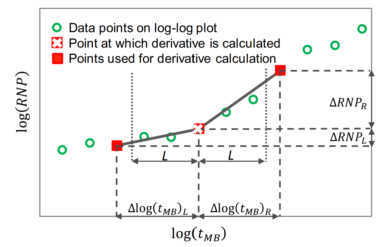
Fig. 2: Bourdet derivative

It is different from a weighted central difference in the way that it uses a constant log-cycle window size, L, on both sides of the point of derivation. A weighted central difference, on the other hand, uses a constant index step size, e.g. i-5 and i+5 for step size of 5, on each side of the point of derivation. The window size, L, represents the log-cycle fraction used to control the amount of smoothing. Typical values are 0.01 to 0.2. The default L in whitson⁺ is 0.2. The larger the L value, the more smoothing.

The Bourdet algorithm implemented in whitson⁺ was provided by Behnam Zanganeh.

1.7.3. Weighted Central Difference

The weighted central difference is given by,

$$\begin{equation} RNP' = \frac{\frac{RNP_L}{\Delta ln(t)_L}\Delta ln(t)_R + \frac{RNP_R}{\Delta ln(t)_R}\Delta ln(t)_L}{\Delta ln(t)_L + \Delta ln(t)_R} \end{equation}$$

where the \(L\)-subscript refers to the index to the left with a constant step size, \(S\), i.e. \(i-S\) and the \(R\)-subscript refers to the index to the right with a constant step size, \(S\), i.e. \(i+S\).

1.7.4. Central Difference

This is the naive implementation, given by three points per derivative for central difference in the following manner

$$\begin{equation} t\frac{RNP}{\delta t} = t_i\frac{RNP_{i+1}-RNP_{i-1}}{t_{i+1}-t_{i-1}} \end{equation}$$

1.7.5. Derivatives in Material Balance Time

Because of noise in real field data, material balance time may not be in sequence. This might cause problems in derivative calculations. Hence, the data must be sorted in terms of increasing material balance time prior to calculating the derivative. The following procedure, adapted from Samandarli et al.(2012), is used for this purpose.

1. RNP and material balance time \((t_c)\) are calculated at each real time step.
2. RNP and \((t_c)\) are sorted in increasing order of material balance time, with repeat material balance times eliminated.
3. The RNP derivative, RNP', is then calculated using the sorted data.

1.8. RTA Integrals

In the case of complex and noisy data, Blasingame et al. [1] introduced the concepts of pressure-integral and pressure-integral difference, which have become essential tools for the scrutiny of well-test data through type-curve analysis. Similarly, McCray (1990) presented the idea of the rate-integral and rate-integral derivative, which was utilized by Blasingame and his students and colleagues for type-curve analysis of production data in various publications.

1.8.1. The Rate Normalized Pressure (RNP) Integral

The use of the RNP integral $\left(IRNP\right)$ and its derivative $\left(IRNP'_R\right)$ was suggested by Chu et al. [6] for the study of flow-regime signature in the Wolfcamp shale. For liquids, the equations are written as follows:

$$\begin{equation} \label{eq:RTA-integral} IRNP=\frac{1}{t_{MB}}\int_{0}^{t_{MB}}\frac{p_i-p_{wf}(\tau_{MB})}{q(\tau_{MB})}d(\tau_{MB}) \end{equation}$$

$$\begin{equation} \label{eq:RTA-integral-derivative} IRNP'_R = \frac{dIRNP}{dln(\tau_{MB})} \end{equation}$$

The integral can be calculated using various time functions (real time or linear superposition time); here it is presented in material balance time for illustration.

As with $\left(RNP\right)$ and $\left(RNP'_R\right)$, the calculations for $\left(IRNP\right)$ and $\left(IRNP'_R\right)$ can be applied to gases through inclusion of gas pseudovariables.

1.8.2. Discrete Calculation

The discrete form of Eq. \eqref{eq:RTA-integral} is expressed in the following manner: $$\begin{equation} \label{eq:RTA-integral-discrete-form} IRNP=\frac{1}{t}\sum_{i=1}^{n}\left(\frac{RNP\left(t_i\right)+RNP\left(t_{i-1}\right)}{2}\right)\left(t_i-t_{i-1}\right) \end{equation}$$

1.8.3. LFP (A√k) Adjustments

The conversion from a slope to LFP (A√k) while using the RNP integral must be adjusted by 2/3 to ensure that the LFP is calculated correctly from the slope. This follows from integrating the RNP as a function of √t.

$$\begin{equation} RNP = mt^{1/2} + b \end{equation}$$

$$\begin{equation} \int RNP \, dt = \frac{2}{3}mt^{3/2} + bt \end{equation}$$

$$\begin{equation} \frac{\int RNP \, dt}{t} = \frac{2}{3}mt^{1/2} + b \end{equation}$$

When turning on the integral function, this correction is applied

1.9. Flow Regimes

To understand why it is important to account for uneven fracture spacing, we review the three relevant flow regimes in tight unconventional reservoirs.

1. Infinite acting flow, often referred to as transient flow, is the flow regime that ends as the pressure transient reaches one reservoir boundary.

2. Transitional flow is the flow regime that starts as the pressure transient reaches one reservoir boundary and ends when the pressure propagation reaches all reservoir boundaries.

3. Boundary dominated flow (∂p/∂t=constant at all locations), also called pseudo-steady state, is the flow regime that starts as the pressure propagation reaches all reservoir boundaries. It occurs when all outer boundaries of the reservoir are no-flow boundaries. These boundaries can be both sealing faults and nearby producing wells or fractures. During this period, the change in pressure at any place in the reservoir decreases at a constant rate. The reservoir is said to behave as a "tank".

For a well geometry with uneven fracture spacing, the flow regime is 1) infinite acting until the boundary between the fractures with the smallest spacing is observed, 2) thereafter it is transitional flow until the boundary between the fractures with the largest spacing is observed, and 3) after that it is in full boundary dominated flow.

1.10. Difference between Classical and Fractional RTA

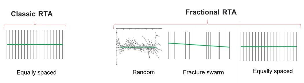
Fig. 3: Visual of the difference between classic RTA and fractional RTA. Courtesy: Jorge Acuna.

In whitson⁺, we distinguish between classical RTA and fractional RTA. Classical RTA solves for equally spaced fracture networks and resolves LFP = A√k = $Ak^{0.5}$ ($\delta$ = 0.5). Fractional RTA solves for a complex system of fractures and resolves LFP = $Ak^{\delta}$ (any value of $\delta$). A visual representation of the difference is shown in Fig. 3. Acuna's (2016, 2020) $\delta$-parameter is a measure of how "uneven" the fracture spacing is. For infinite conductive fracture, the $\delta$ value is between 0 (highly uneven fractures) and 0.5 (even fracture spacing).

1.11. Estimate \(\delta\) from Production Data

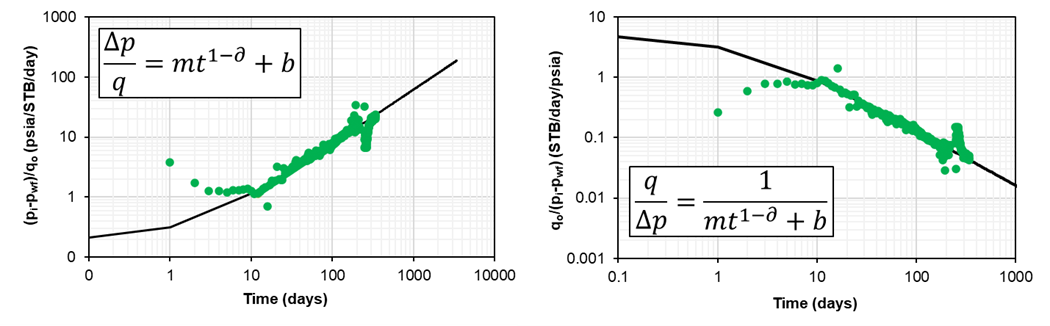
Fig. 4: Rate Normalized Pressure (RNP) as a function of time (left) and Pressure Normalized Rate (PNR) as a function of time (right) on a log-log scale

An estimate of $\delta$ can be obtained by plotting rate normalized pressure (RNP) versus time, [$\frac {(p_i-p_{wf})}{q} \text {vs.} t$] on a log-log scale, followed by a best fit of the power-law function provided by:

$$\begin{equation} \label{eq:delta} \frac{\Delta p}{q}=mt^{1-\delta}+b \end{equation}$$

Alternatively, one can plot and fit the reciprocal, i.e., the pressure normalized rate (PNR) versus time [$\frac{q}{(p_i-p_{wf})}$ vs. $t$]. Examples of these plots are provided in Fig. 4. For single-phase oil cases (e.g., \(p_{wf}\) > \(p_{b}\), little/no water) oil rates can be used. For multiphase systems (\(p_{wf}\) < \(p_{sat}\) and/or significant water production), it is recommended to use total reservoir rates (surface oil, gas and water rates converted from surface to reservoir volumes using proper PVT and pressures). For single-phase gas (dry/wet gas or \(p_{wf}\) > \(p_{dew}\), little/no water) one can use gas rates and pseudopressure.

1.12. Physical significance of \(\delta\)

In material balance time,

Flow Parameter $\delta$	Flow Regime / Interpretation
$\delta$= 1	indicates radial flow
$\delta$ = 0.75	indicates bi-linear flow
$\delta$ > 0.5	indicates low conductivity fracture systems
$\delta$ = 0.5	indicates infinite acting linear flow
0 < $\delta$ < 0.5	indicates transitional flow
$\delta$ = 0	indicates boundary dominated flow

Why do we generally prefer to use material balance time for analyzing the $\delta$-parameter in Fractional RTA?

• Infinite acting linear flow, in real time and material balance time, exhibits a $\delta$ of 0.5.
• In material balance time, transitional flow will exhibit a $\delta$ between 0 and 0.5 and boundary dominated flow yields $\delta$ = 0 (a unit slope on the RNP vs MBT plot).
• In real time, however, transitional flow $\delta$ ranges from 0.5 to $-∞$ and boundary dominated flow yields $\delta$ = $-∞$. Hence, using this range to analyze flow regimes may be impractical for most people.

1.13. Relationship between \(\delta\) and Arps' b-factor

There is a relationship between the $\delta$-parameter and Arps' b-factor. $$\begin{equation} \label{eq:b_to_delta} \delta = 1 - \frac{1}{b} \end{equation}$$ $$\begin{equation} \label{eq:delta_to_b} b = \frac{1}{1-\delta} \end{equation}$$

Remember

If you use the $\delta$-parameter to constrain b-factors used in DCA, you must resolve the $\delta$-parameter in real time (not material balance time).

1.14. Governing Equations

The equation for rate normalized pressure is written as $$\begin{equation} \label{eq:delta2} \frac{\Delta p}{q}=mt^{1-\delta}+b \end{equation}$$

where \(m\) is the slope of RNP versus time.

For oil: $$\begin{equation} \label{eq:m-oil} m=\frac{0.468}{0.001055^{\delta}}\frac{24^{1-\delta}}{\Gamma\left(\delta\right)\left(1-\delta\right)}\frac{B_o}{4hx_fk^\delta}\frac{\mu_o^\delta}{\left(\phi c_t\right)^{1-\delta}} \end{equation}$$

For gas: $$\begin{equation} \label{eq:m-gas} m=\frac{4.716}{0.001055^{\delta}}\frac{24^{1-\delta}}{\Gamma\left(\delta\right)\left(1-\delta\right)}\frac{T_R}{4hx_fk^\delta}\frac{\mu_g^{\delta-1}}{\left(\phi c_t\right)^{1-\delta}} \end{equation}$$

Constant flowing pressure solution: $$\begin{equation} \label{eq:cp-solution} \frac{p_i-p_{wf}}{q}=\frac{\pi}{2}mt^{1-\delta}+b \end{equation}$$

Constant rate solution: $$\begin{equation} \label{eq:cr-solution} \frac{p_i-p_{wf}}{q}=mt^{1-\delta}+b \end{equation}$$

For gas, use pseudopressure to substitue \(p_i\) and \(p_{wf}\) in Eqs. \eqref{eq:cp-solution} and \eqref{eq:cr-solution}.

$$\begin{equation} \label{eq:LFP} LFP'=Ak^\delta \phi^{1-\delta}=4n_fx_fhk^\delta\phi^{1-\delta} \end{equation}$$

The equation for skin (S) is related to the intercept b, and given by

$$\begin{equation} \label{eq:skin_frta} S=b\frac{khx_f}{221.8\mu} \end{equation}$$

Here \(x_f\) is the cumulative length of the fracture.

1.15. Solving for LFP

One can solve for LFP by knowing the estimates of m (coefficient) and $\delta$ (slope) obtained from the rate normalized pressure (RNP) versus time plot, [(pi-pwf)/q vs. t on a log-log scale].

For oil: $$\begin{equation} \label{eq:LFP-acuna-oil} LFP=\frac{0.468}{0.001055^{\delta}}\frac{24^{1-\delta}}{\Gamma\left(\delta\right)\left(1-\delta\right)}\frac{B_o\mu_o^\delta}{\left(\phi c_t\right)^{1-\delta}}\frac{1}{m}\end{equation}$$

For gas: $$\begin{equation} \label{eq:LFP-acuna-gas} LFP=\frac{4.716}{0.001055^{\delta}}\frac{24^{1-\delta}}{\Gamma\left(\delta\right)\left(1-\delta\right)}\frac{T_R\mu_g^{\delta-1}}{\left(\phi c_t\right)^{1-\delta}}\frac{1}{m} \end{equation}$$

1.16. \(\delta\)-parameter and Radial Flow

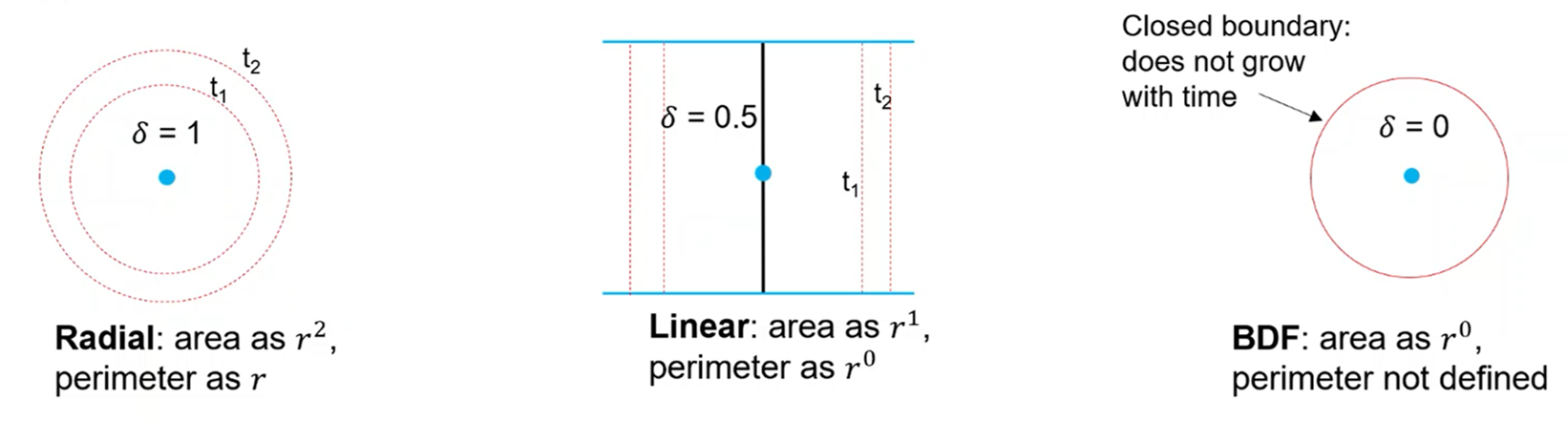
Fig. 5: Visual showing $\delta$=1 for radial flow. Courtesy: Jorge Acuna.

$\delta$=1 would indicate radial flow, $\delta$=0.5 would indicate linear flow and $\delta$=0 indicates boundary dominated flow. Another way to think about it is that the flow type depends on how the drainage area and the perimeter (area perpendicular to flow) grow with time.

References

[1] Acuna, Jorge A. "Analytical Pressure and Rate Transient Models for Analysis of Complex Fracture Networks in Tight Reservoirs." Paper presented at the SPE/AAPG/SEG Unconventional Resources Technology Conference, San Antonio, Texas, USA, August 2016.

[2] Acuna, Jorge A. "Rate Transient Analysis of Fracture Swarm Fractal Networks." Paper presented at the SPE/AAPG/SEG Unconventional Resources Technology Conference, Virtual, July 2020.

[3] Carlsen, Mathias Lia, and Curtis Hays Whitson. "Numerical RTA Extended to Complex Fracture Systems: Part 1." Paper presented at the SPE/AAPG/SEG Unconventional Resources Technology Conference, Houston, Texas, USA, June 2022.

[4] Samandarli, Orkhan , Valbuena, Ernesto , and Christine Ehlig-Economides. "Production Data Analysis in Unconventional Reservoirs with Rate-Normalized Pressure (RNP): Theory, Methodology, and Applications." Paper presented at the SPE Americas Unconventional Resources Conference, Pittsburgh, Pennsylvania USA, June 2012.

[5] Palacio, J.C. and Blasingame, T.A. "Decline Curve Analysis Using Type Curves; Analysis of Gas Well Production Data." Paper Presented at the SPE Rocky Mountain Regional/Low Permeability Reservoirs Symposium, Denver, Colorado, April 12-13.

[6] Chu, W.–C.. –C., Pandya, N. D., Flumerfelt, R. W., and C.. Chen. "Rate-Transient Analysis Based on the Power-Law Behavior for Permian Wells." SPE Res Eval & Eng 22 (2019): 1360–1370.