Nodal Analysis - IPR / VLP
1. Overview
The Nodal Analysis feature provides a simple way of evaluating whether the current well configuration produces the reservoir fluids efficiently, or if a different well configuration would increase well performance.
1.1. Selection of Production Test Date and Creation of IPR
Choose the production test date as shown below. This is used to calculate the Productivity Index, \(J\), at a point in time from the well's production history.
Selection of the desired date here will automatically populate the Production Data section right below it with pressures and rates from the well's production history on the selected date.
Next, the Productivity Index Data section is automatically populated from the date selection as follows:
- Liquid rate, GOR and WOR are calculated based on the selected production test date input and the associated rates for that date.
- BHP is fetched from the Bottomhole Pressure module.
- Reservoir pressure is fetched from the Multiphase Flowing Material Balance module.
- Saturation pressure is fetched from the PVT module.
If the BHP, MFMB, or PVT analyses are not done for the well, these fields will be blank and the values must be specified manually for IPR generation.
The productivity index is calculated at the liquid rate (oil + water) and the specified pressures using the Vogel IPR as outlined above.
1.2. Changing the Wellbore Configuration & Creating VLPs
The main intent of this feature is to provide a 'What-if' tool for analyzing different well configurations. The active configuration on the production test date is considered the default or current well configuration and this can be compared against a new wellbore configuration.
- Use the Modify Cases button to set the existing and new well configurations and see them side-by-side, which helps compare inputs.
- You can fix the Casinghead Pressure and Tubinghead Pressure to a constant for both configurations to generate a VLP specific to this combination of parameters for the purpose of comparing them.
- Once the well configurations are saved, you can choose the BHP correlation and select which configuration to run for each case to compute the VLP.
- The new VLP curves are generated when you click Save and then Run on each case in the table.
This step generates various VLP curves - one for each well configuration, representing the deliverability of the well under each configuration's constraints, and one for the current case under current well settings.
The difference in these VLP curves, based on where they intersect the IPR, indicates the difference in stable production rates expected from each wellbore configuration by reading the gas rates plotted on the x-axis at the point of intersection.

In the example shown in the gif above, we see a variance in production rates depending on which tubing diameter is used for the well.
1.3. Saving Different Cases
In reality, you may have more wellbore configurations than the number shown in the gif to choose from for a particular well. You can save each new wellbore configuration independently as a case, allowing you to compare up to ten different wellbore configurations at once.
- Click on Modify Cases in the top right corner.
- Click Add/Edit Well Configuration to change any existing configurations or to create new ones.
- Edit the new case with corresponding Casinghead and Tubinghead Pressure, production ratios, and wellbore configuration.
- Click Save on the bottom-right. All the saved cases will appear in the VLP Cases table above the IPR-VLP plot.
- You can activate the relevant cases to be shown in the IPR-VLP plot by using the checkbox for each case.
1.4. IPR and VLP Assumptions
- The pseudopressure is rigorously calculated to generate C&n IPR.
- A fixed value of \(n = 1\) is assumed for the C&n IPR.
- "Vogel (Oil + Water)" provides an IPR for surface liquid rate versus pressure. This curve is created from the sum of the Vogel IPR applied to the oil and a straight-line IPR applied to the water phase.
1.5. VLP calculations with quiet side option
When using the quiet side for bottomhole pressure (BHP) calculations, a flat vertical lift performance (VLP) in nodal analysis is typically observed. This is due to the assumption that the quiet side represents a single-phase column that is not flowing. In this scenario, the only factor contributing to the pressure drop is the gravity component of the gas column, particularly down to the end of the tubing.
In cases where there is a short distance (less than 100 feet) between the end of the tubing and the top perforation, this small section is the only place where a change in the calculated BHP versus rate will occur. As a result, the VLP appears flat, as it shows the BHP calculated for different rates, and for the quiet side, the BHP is essentially independent of the flow rate.
For more details on how the calculation on the quiet side works, please refer to Static (Quiet) Side.
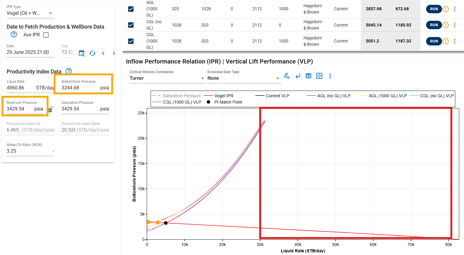
1.6. Incomplete VLP Curves
High flow rates through narrow tubing can cause the VLP solver to fail at higher rates. As tubing narrows or flow increases, the pressure drop per foot becomes steeper. The solver calculates VLP by stepping through flow rates from the IPR curve, but if the pressure gradient is too steep, the solver’s step size becomes too large to maintain numerical stability, leading to missing points on the VLP curve. The narrower the tubing, the lower the flow rate limit before the solver hits this failure point. Also the lower the wellhead pressure, the lower the limit, because the gas occupies more space and causes a larger pressure drop.
High Flow Rate Example
These issues occur when the IPR predicts very high flow rates—for example, 30,000 STB/day of liquid as shown below. Such high rates are difficult to handle in the tubing and may indicate the IPR is unrealistic, especially if reservoir pressure is close to bottomhole pressure. Increasing reservoir pressure can produce more reasonable rates and resolve the issue.
Key points for users:
- Narrower tubing or lower wellhead pressure lowers the maximum flow rate before failure occurs.
- Extremely high IPR rates (e.g., tens of thousands of STB/day) can trigger this issue.
- The solution is to use a more reasonable IPR.
- The failed VLP points likely won't matter, as they represent very high rates and high BHPs (mostly larger than reservoir pressure) — meaning they aren't physically meaningful in practice.
1.7. Multi-point Sampling for IPRs
Select a more representative IPR curve by minimizing the impact of outliers. A 10-day history sample is used to illustrate the range of possible IPRs.
Show Additional Points on the Graph - You can display liquid rate and bottomhole pressure (BHP) points from other dates on the IPR/VLP graph. It helps you compare well performance on different days, all within the same plot. Each point is clickable. Selecting one will automatically update the graph to that date’s IPR/VLP inputs and reposition the cursor to show the corresponding liquid rate and BHP. This makes it easy to explore trends, spot high-performance periods, and assess how current operations compare to past conditions.
Show Additional IPR Curves on the Graph - You can overlay IPR curves from other dates on the same graph, helping you visualize how inflow performance can change with respect to time. Each additional IPR curve gives context for evaluating current well conditions relative to past performance. This is useful for spotting inflow degradation, improvement, or validating the effectiveness of interventions.
1.8. Average IPR
Build a representative IPR by averaging production over a user-defined date window. This smooths noise and gives a stable curve for VLP comparisons and case screening.
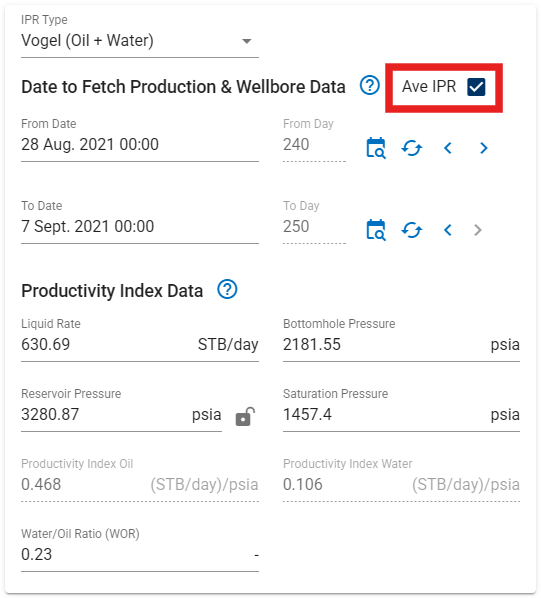
- In IPR/VLP, open the IPR panel and select Average IPR.
- Set Start Date and End Date for the averaging window.
- Choose streams and pressures to include. The tool computes liquid rate (oil + water), GOR, WOR, and uses BHP, reservoir pressure, and saturation pressure for the averaged point.
- Generate the Average IPR and plot it with your VLPs.
1.9. Extend VLP Max
Calculate and plot VLP beyond the max IPR rate (AOF) to enable broader operational analysis and predictive evaluations.
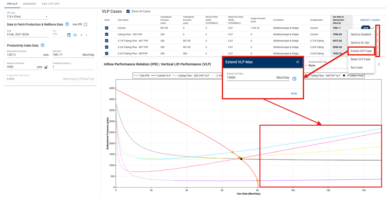
- In VLP Cases, open the options menu and select Extend VLP Max.
- Enter the new maximum rate and click Run.
- The VLP curve is extended and plotted beyond the IPR limit.
1.10. Erosional velocity/rate models
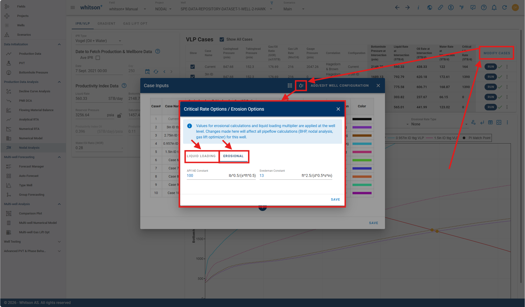
- Access by going to VLP Cases,
- Click Modify Cases → Edit Well Data
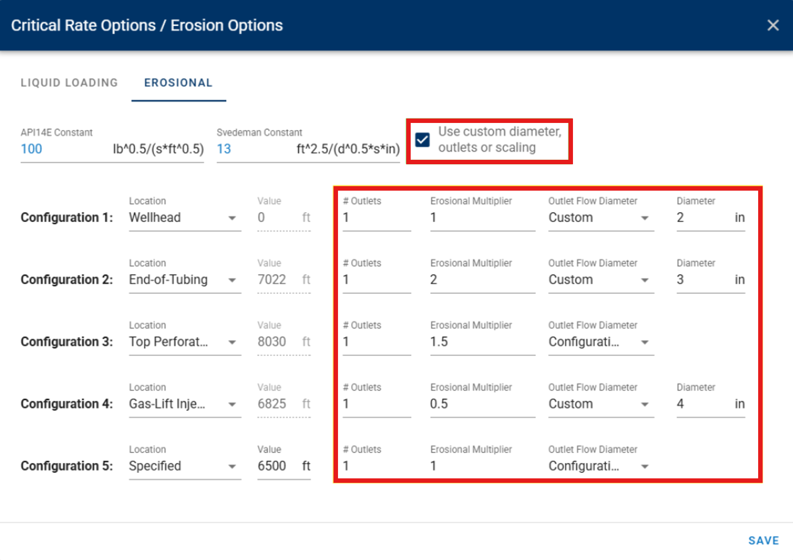
Customizable erosional velocity/rate models add flexibility to adjust diameter, outlets, or scaling.
-
Check Use custom diameter, outlets or scaling to enable the configuration fields
-
For each listed Configuration row:
- Location: select where the erosional check applies (e.g., Wellhead, End-of-Tubing, Top Perforation, Gas-Lift Injection, Specified).
- Value: enter the depth/value (ft) for the selected location.
- # Outlets: set the number of outlets used for the erosional check.
- Erosional Multiplier: enter a multiplier used in the erosional calculation.
- Outlet Flow Diameter: choose Custom to type a Diameter (in), or choose Configuration to use the configuration’s diameter.
-
Be sure to click Save to apply.
2. Theory
2.1. Reservoir IPR
2.1.1. Straight-Line IPR
The reservoir inflow performance relation (IPR) represents a simple explicit relationship between the surface rate, \(q_{\bar{p}}\), of phase \(p\), and the flowing bottomhole pressure \(p_{wf}\). The simplest IPR is the linear relationship
where \(p_R\) is the average reservoir pressure, \(J\) is the productivity index, and \(p_{wf}\) can vary in the range \(0 \leq p_{wf}\leq p_R\). The lower bound, \(p_{wf}=0\), is a theoretical point known as the absolute open flow (AOF) point where \(q_{\bar{o}}=q_{\bar{o},max}\). The upper bound, \(p_{wf}=p_R\), represents a shut well where \(q_{\bar{o}}=0\).
For a vertical well that fully perforates a cylindrically shaped homogenous reservoir, it can be shown, assuming the product \(\mu_oB_o\) is only slightly pressure dependent, that the productivity index is equal to
2.1.2. Vogel IPR
Oil and Gas Flow
Saturated Reservoir Conditions (\(p_R\leq p_{b}\))
The straight-line IPR is only valid for slightly-compressible fluids, such as undersaturated oils and water. For an undersaturated oil, continued production will ultimately bring the average reservoir pressure, \(p_R\), below the initial bubblepoint pressure, \(p_{b}\), at which gas starts coming out of solution. The free gas phase will make the total compressibility of the system increase rapidly, and the straight-line (slightly compressible fluid) assumption is no longer representative. To account for the release of solution gas, Vogel[1] suggested an IPR on a normalized form:
Assuming a straight-line IPR, tangent to the Vogel IPR at \(p_{wf}=p_R\), it can be shown that the maximum oil rate of the Vogel IPR, \(q_{\bar{o},max}\), is:
Undersaturated Reservoir Conditions (\(p_{b} < p_R\))
For undersaturated oils (\(p_{b}<p_R\)), it is normal to combine the straight-line IPR and Vogel IPR in the same plot to show the effect of gas coming out of solution as the flowing bottomhole pressure becomes less than the bubblepoint pressure. To achieve this, the two IPRs are connected at the bubblepoint pressure. The Vogel IPR is used in the pressure range from 0 \(p_{b}\), and the straight-line IPR is used in the pressure range from \(p_R\) to \(p_{b}\). The combined IPR can be expressed as:
Oil, Gas, and Water Flow
The Vogel IPR accounts for the effect of released solution gas (i.e., the effect of free gas flowing together with the oil). To get the rates of both phases at a given \(p_{wf}\), the oil rate is calculated by the IPR, and the gas rate is calculated by \(q_{\bar{g}}=q_{\bar{o}}R_{p}\), where \(R_p\) is the producing gas/oil ratio assumed independent of \(p_{wf}\). In the case of three-phase flow (oil, gas, and water), the simplest case would be to calculate the water rate from \(q_{\bar{w}}=q_\bar{o}F_{wp}\), where \(F_{wp}\) is the producing water/oil ratio assumed to be independent of \(p_{wf}\).
However, this would lead to the water production behaving as if it has significant gas in solution (curved IPR for the water phase). It is arguably more accurate to handle the water phase separately by its own straight-line IPR. The liquid-phase (oil + water) IPR will then be the sum of the straight-line IPR for water and Vogel IPR for oil. For an undersaturated oil reservoir with free water flowing, the following is used as the liquid-rate IPR.
Here is an example that compares the results of manual calculations using these equations with those obtained from whitson+
Vogel IPR Curve Calculation Example
2.1.3. C&n IPR
Pressure-Squared Approximation
The Vogel IPR is applied to fluid systems that initially are undersaturated oils. For fluid systems that initially are gases, the C&n IPR, sometimes referred to as the "back-pressure equation", is used.
Rawlins and Schellhardt[2] performed multirate deliverability tests on over 500 gas wells and noted that the difference between the average reservoir pressure squared and the flowing bottomhole pressure squared (i.e. \(p_R^2 - p_{wf}^2=\Delta p^2\)) plotted against the corresponding stabilized flow rates produced a straight line in a log-log plot. Hence, the IPR was suggested to be
The exponent represents the effect of high-velocity inflow to the well (i.e., the effect of non-Darcy turbulent flow).
- \(n=1\) for when the flow is characterized by Darcy's equation.
- \(0.5 \leq n \leq 1\) for when the flow is characterized by non-Darcy effects and turbulence.
The coefficient \(C\) is a measure of deliverability accounting for primarily the drainage area and permeability.
Fetkovich[4] argued that the pressure-squared C&n IPR could also be used for saturated oils, as it is very similar to the Vogel IPR equation for \(n = 1\). The C&n equation with \(n=1\) can be written as
which results in an IPR that's a little more conservative than Vogel's. Field data may often be matched equally well to both IPRs, making the C&n equation a more general IPR as it may be applied to both saturated oils and gases.
Well-test procedures for determining \(n\)
The multirate tests used to generate the straight line plots in log-log pseudopressure vs rate consist of a series of pressure vs rate measurements, which may be:
- Flow-after-flow tests - Producing the well at stabilized flow rates and pressures. Rawlins and Schellhardt used this but it may be practically impossible to test the well long enough to obtain stabilized data for low-permeability gas wells.
- Isochronal tests - Producing the well at different flow rates with flowing periods of equal duration. Each flow period is separated by a shut-in period long enough to allow the bottomhole pressure to stabilize at the average reservoir pressure (again, not possible in low-permeability reservoirs). They also need an extended stabilized flow point.
- Modified isochronal tests - Overcome the limitation of obtaining stabilized data for low-permeability wells by modifying the isochronal test to require shut-in periods longer than or equal to the flow periods separating them. They are less accurate than isochronal testing.
- Transient tests - Require estimates of drainage area and shape, additional reservoir and fluid properties, and are hence complex, but they eliminate the need for stabilized data.
Such high-quality multirate test data are rarely available for all wells, so it may be hard to determine the deliverability exponent. It has been shown by Golan and Whitson[3] and field data from gas wells that the value of n only varies slowly and can be assumed to be roughly constant over the life of the well to simplify calculations and avoid the use of rock and fluid properties to estimate future deliverability.
Rigorous Handling with Pseudopressure
Gas well performance through the pressure-squared approximation is only valid at low reservoir pressures. To rigorously calculate the flow at all pressures, it is necessary to use the pseudopressure defined as:
In the C&n IPR, the pressure-squared terms are simply replaced by the pseudopressure, yielding
Non-dimensional form of the backpressure equation using AOF rate
This backpressure equation is written in normalized form with AOF rate and squared pressures to develop the IPR equation for gas wells in dimensionless form as
We can write the same equation in terms of gas pseudopressures as:
Note on Constant Productivity Index, \(J\) and stable inflow performance
Stable inflow performance—constant \(J\)—requires the condition of pseudosteady-state (PSS) / boundary-dominated flow. Simply stated, PSS represents the condition when the entire drainage volume of the well contributes to production. In high permeability formations, this may happen instantaneously but in low permeability formations, the flow may be infinite acting for years in which case, expecting a stabilized IPR is not practical. If the reservoir has not reached PSS yet, then both \(J\) and \(C\) will be time-dependent and consequently keep shrinking the IPR envelope towards the origin until stable values are achieved.
2.3. Calculating the Well PI
To compute IPR of a well, it is necessary to provide a test point \((q_{\bar{j},test}, p_{wf,test})\) for phase \(j\) to compute the productivity index \(J\) for the Vogel IPR, and the deliverability constant \(C\) for the C&n equation.
2.3.1. Vogel (Oil + Water) PI
For oil phase using the Vogel IPR, the productivity index \(J_o\), may be calculated in a few different ways, depending on the conditions of the test point.
If the test occurs at the conditions \(p_{bi}<p_{wf,test}<p_R\), then \(J_o\) is computed from first definition of the combined IPR in Eq. (\ref{eq:combined})
If the test occurs at the conditions \(p_{wf,test}<p_{bi}<p_R\), then \(J_o\) is computed from the second definition of the combined IPR in Eq. (\ref{eq:combined})
For the water phase, the test point \((q_{\bar{w},test},p_{wf,test})\) is used to compute the water PI, \(J_w\), from a straight-line IPR
The liquid rate as a function of flowing bottomhole pressure is then computed as:
2.3.2. C&n (Gas) PI
For the gas phase using the C&n IPR, the deliverability constant \(C\), is calculated by
where we have assumed \(n=1\). If \(n\) is also unknown, then at least two test points are required.
2.4. Well VLP
The Vertical Lift Performance, VLP (also referred to as Tubing Performance Relationship, TPR) describes the pressure drop associated with lifting the fluid at a given rate through the given wellbore configuration at fixed tubing head pressure or casing head pressure.
The VLP takes into account the following pressure elements at the bottomhole, across the range of possible production rates, to determine the deliverability of the well in combination with what the reservoir can deliver (i.e. the IPR) -
- Backpressure exerted at the surface from the choke and wellhead assembly—Wellhead pressures
- Hydrostatic pressure due to gravity and the elevation change between the wellhead and the intake to the tubing—Fluid properties and deviation survey
- Friction losses, which may include irreversible pressure losses due to viscous drag and slippage—Current or planned wellbore configuration and rates
The VLP is only valid for a specific set of well data.
Changing wellhead pressure, gas/liquid ratio, i.e., PVT, or tubing dimensions in wellbore configurations will change the VLP and will require the construction of a new curve.
If the tubing intake pressure calculated from the VLP intersects the bottomhole pressure from the IPR curve, the rate at the point of intersection determines the deliverability of the well and this is the rate of natural, stable flow that can be expected from the particular well in this configuration.
The point of intersection gives the natural flow rate by reading the rate axis on the nodal analysis plot.
If there is no intersection, the given backpressure and wellbore configuration will be unable to naturally deliver the fluid to the surface from the tubing intake.
What if my IPR and VLP intersect in two places?
This is likely for certain multiphase mixtures and configurations. One represents a stable flow condition and the other is an unstable one. Mathematically, the stable point of natural flow exists when the two performance curves intersect with slopes (derivatives) of opposite sign. If the two performance relations intersect with slopes at the point of intersection of similar sign, the well is in unstable equilibrium and only a small change in rate may cause the system to change its state of equilibrium, either killing the well or moving it toward the stable point of natural flow.
3. Choke
The choke setting represents a pressure restriction point in the wellbore or surface facility and determines the pressure drop between two points in the system. This is typically between the wellhead and surface flowline, or at a specified downhole depth. Each wellbore configuration includes one choke settings such as choke coefficient, choke depth, and choke size.
What is Choke Coefficient?
The Choke Coefficient is a correction factor used to account for vena contracta effects and irreversible energy losses. This coefficient can be estimated using single-phase valve coefficients provided in manufacturer datasheets, or more accurately determined through field calibration with measured field data.
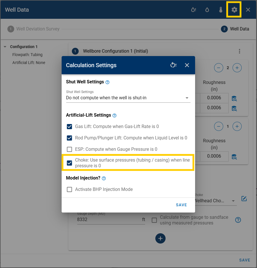
When configuring a choke in whitson+, it is important to understand which pressure reference is required depending on where the choke is located:
-
For wellhead chokes, the line pressure should be used. Otherwise, you can choose to fall back on tubing or casing pressure using the toggle shown below. Moreover, note that the choke depth is always zero and the choke size is fetched from production data.
-
For Downhole Choke, the default tubing or casing pressure is used. The choke depth and size (opening) are required. If choke size changes with time, user can add new configurations and edit the size for those configurations.
Operational Envelope
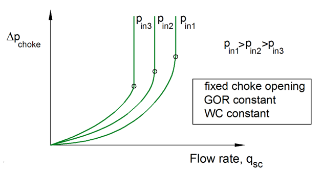
A fixed opening wellhead or bottom-hole choke will display the performance curve (pressure drop vs. surface oil or gas rate), shown in the figure below.
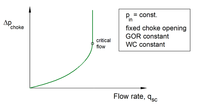
This curve is generated by keeping the inlet pressure, GOR, and WC constant, while changing the downstream pressure from the inlet pressure value to atmospheric conditions (see the sequence plotted in the animation below).
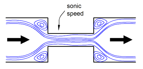
The pressure drop across the choke increases in a non – linear manner when the rate is increased. However, there is a point where it is not possible to increase the rate further (i.e., the pressure downstream the choke does not impact the rate flowing through the choke). This is because the fluid velocity at the throat of the choke has reached the sonic velocity. This typically occurs when the pressure ratio is between 0.5-0.6.
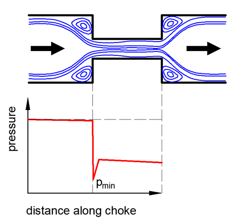
The figure below shows the behavior of pressure along the axis of a bean choke. Note that pressure drops suddenly when the flow encounters the contraction point. In gas-dominated flows this sudden pressure reduction can cause cooling (due to the Joule-Thomson effect), liquid condensation and ice formation (in the presence of free water).
The figure below shows the performance curve of the choke when the inlet pressure is varied. The pressure drop at which the critical flow is reached increases proportionally with the inlet pressure: . Changes in GOR and WC give a similar variation of the performance curve.
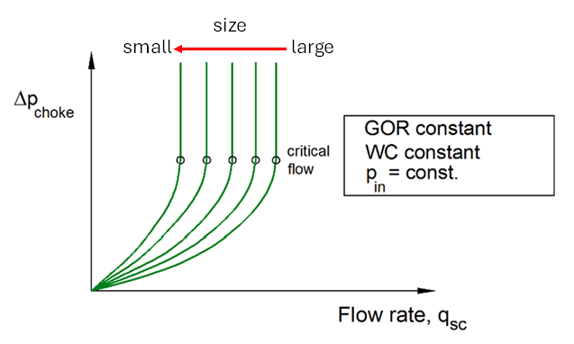
The figure below shows the choke performance curve for 5 different choke openings. A smaller opening will provide a larger pressure drop than a larger opening, and critical flow will be reached at lower flow rates.
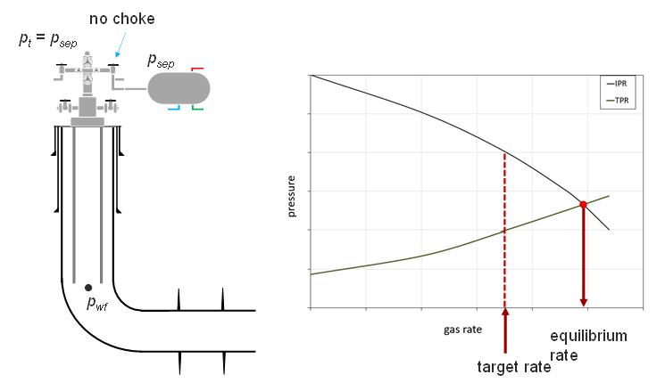
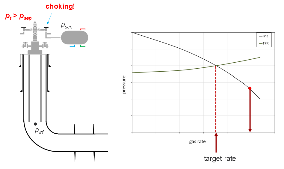
Choke Planning Using Nodal Analysis
Consider the situation shown in the figure below. A nodal analysis is performed at the bottomhole on a well with no wellhead choke. The equilibrium rate is higher than the target rate; therefore, choking is required.
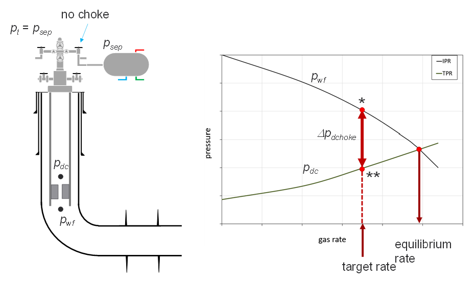
If a bottom-hole choke is used, the choke must drop the pressure from the pressure available from the reservoir (marked with * in the figure) to the pressure required to flow to the surface through the tubing (marked with ** in the figure).
Another alternative is to use wellhead choking (shown in the figure below). In this approach, wellhead choking increases the tubing head pressure and “shifts” the TPR up, moving the intersection to the left.
Choke Modeling
Chokes are often modeled by integrating the differential version of the momentum equation between the choke inlet and the throat and assuming no friction or localized losses between these two points. Due to the convergence of the flow, the effective throat cross-section area (often referred to as vena contracta) is not exactly equal to the throat cross-section area (), thus a correction factor () is introduced () and is often varied in the range (0,1] such that the model predicts accurately measured data.
The one-dimensional momentum equation in differential form for liquid-gas flow, neglecting friction and localized losses, is:
where is holdup, is velocity, is density, and pressure.
The whitson+ model assumes liquid and gas travel at the same velocity (mixture velocity, , equal to the sum of local rates of oil, gas and water divided by cross-section area). Then, the equation above is integrated between the inlet and the throat, while neglecting inlet velocity, to obtain:
is the homogeneous mixture density, defined as:
where is the gas mass fraction, and , are the gas and liquid phase densities, respectively.
Calculation Details
In all whitson+ applications like bhp calculations and nodal analysis, rate across and pressure downstream the choke are known, and it is desirable to find inlet pressure.
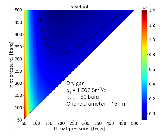
The equation is solved by computing numerically the homogeneous density integral, assuming isothermal flow and thermodynamic equilibrium. However, there is some care to be exercised about the pressure value to employ at the throat.
When operating in the subcritical regime, the pressure downstream of the choke is usually employed to approximate the pressure at the throat, assuming there is very little pressure recovery after the throat. When operating in the critical regime, the pressure measured downstream of the choke is lower than the pressure at the throat and is initially unknown. The main challenge is that often it is not known beforehand if the choke is operating in the critical or subcritical regime, so the calculation requires some trial and error.
As an example, consider the flow of dry gas through a choke, outlet pressure equal to 50 bara, inlet temperature 80 °C. The figure below shows the value of the residual of the choke model for a rate of 1e6 Sm3/d, and for several combinations of inlet pressure and throat pressure values, from 50 bara to 500 bara. Cases where the inlet pressure is lower than the throat pressure are discarded. The black line is the inlet-throat pressure combinations where the residual is zero (potential solutions to the choke model). The physical solution is the minimum point in the black curve. When the minimum lies when the throat pressure is equal to the downstream pressure, the choke operates in the subcritical regime. Otherwise, the choke operates in the critical regime (like in the figure below).
Recommended Practice for BHP Calculations
When estimating BHP, always aim to use the shortest and most reliable pressure path. If there is a wellhead choke, but measured tubing head pressure or casing head pressure is available and considered reliable, it is generally best to ignore the wellhead choke and calculate BHP directly from this surface pressure. Doing so minimizes assumptions, simplifies the pressure path, and improves accuracy.
Preferred Calculation Path:
- Tubing/casing head pressure → tubing/casing pressure drop → bottomhole pressure
This direct approach is preferable to the more assumption-heavy path that includes a wellhead choke:
- Line pressure → wellhead choke pressure drop → tubing/casing head pressure → tubing/casing pressure drop → bottomhole pressure
This distinction is especially important when high-confidence surface pressure data is available — performing wellhead choke calculations in such cases may unnecessarily introduce uncertainty.
When Downhole Gauge Data Available
If a downhole pressure gauge is available, it is best to use that data directly for BHP estimation. This eliminates the need for pressure gradient assumptions and calculations entirely, resulting in the shortest and more reliable output.
When to Use Wellhead Choke-Based Calculations
- Surface pressure is unavailable or unreliable, but line pressure and flow rates are available.
- Line pressure and surface pressure are available, but flow rates are unavailable or unreliable (an iterative approach will be used to adjust rates until the calculated surface pressure matches the measured value)
- Simulating or designing choke strategies for operational optimization, such as evaluating pressure response or production control, erosion mitigation, etc.
Estimating Choke Size from Cv
When working with adjustable chokes, manufacturers often provide a value of flow coefficient Cv for different openings (position, usually in %). whitson+ requires choke size in 1/64 in as input. You can use the following equation to convert from Cv to choke size in 1/64 in:
Manual Calibration of Choke Coefficient (wellhead choke)
If you have values of wellhead pressure, line pressure and rate, you can use them to tune your choke coefficient, such that the accuracy of your choke calculations is improved. To do this, go to the feature "gradient" in the "Nodal Analysis" module. Select the date you want to do the calibration for. Wellhead pressure (either tubing or casing head pressure, depending on the flow path) is an output of the calculation. Adjust the choke coefficient manually until the wellhead pressure output of gradient calculation matches the measured value of wellhead pressure.
Manual Calibration of Choke Coefficient (bottomhole choke)
If you have a bottomhole gauge, you can use it to tune your choke coefficient, such that the accuracy of your choke calculations is improved. To do this, go to the feature "gradient" in the "Nodal Analysis" module. Select the date you want to do the calibration for. The calculation outputs pressure versus depth, and one can read pressure at gauge depth. Adjust the choke coefficient manually until the gauge pressure output of gradient calculation matches the measured gauge value