whitson⁺ - Getting Started

1. Introduction

Complete the steps outlined below to become a certified whitson⁺ user. It includes performing a well performance workflow for three wells with actual production data from the SPE Data Repository . Those certified have the software skills necessary to complete most well performance evaluation projects in tight unconventionals.

Need help?

Send an e-mail to support@whitson.com.

1.1. Before Starting

Make sure you have watched these three videos in the Getting Started part of the manual (click here).

• 1.1 Login (1 min)
• 1.2 Overview of important basics (3 min 30 sec)
• 1.3 Zoom Plots (3 min)

1.2. Create a Project

1. Go to the Project module in the navigation panel.
2. Click ADD PROJECT up to the right.
3. Name the project "your name - whitson certificate".
4. Click SAVE.
5. All steps are shown in the .gif above.

1.3 Upload Well Data

1. Download the relevant data for the three wells →→ here ←←.
2. In the Wells module, click MASS UPLOAD up to the right.
3. Upload relevant data in your project dropping the data file into the MASS UPLOAD frontend.
4. All steps are shown in the .gif above.

1.4 Mass Edit Data

1. In the Wells module, click EDIT ALL up to the right.
2. Scroll to the right and make the Matrix Gamma and Fracture Gamma numbers 2.
3. Click SAVE.
4. All steps are shown in the .gif above.

2. Dry Gas ("Single-phase") Well

Wellname: SPE-DATA-REPOSITORY-DATASET-1-WELL-37-PHEASANT

We will start with a dry gas well, with little water production. In reality, this is the closest we will get to a "single-phase" flow problem. It is a great place to start the learning curve for unconventional well performance.

2.1 PVT

2.1.1 Reservoir Fluid Composition

1. Go to the PVT module in the navigation panel.
2. Open the Reservoir Fluid Composition Input Card
3. Change the Method from "GOR" to "Dry/wet Gas".
4. Input a Gas Specific Gravity (SG) of 0.6.
5. Click SAVE.
6. Check the predicted fluid composition by clicking the "eye icon".
7. All steps are shown in the .gif above.

2.1.2 PVT Table

1. Go to the PVT TABLE tab.
2. Click EXPORT up to the right.
3. Click EXCEL in the dropdown menu to download the table to excel.
4. We'll not use this table, this is just to show you how this is done.
5. This table represents the PVT that will be used for this well.
   It's done automatically - so just sit back and relax (:
6. All steps are shown in the .gif above.

2.2 Production Data

1. Go to the Production Data module in the navigation panel.
2. Click EDIT up to the right.
3. Change the first measured gauge pressure to 4200 psia.
4. Delete all data after 700 days.
   Keyboard shortcut: CTRL + SHIFT + left arrow + down arrow
5. Click SAVE.
6. Does this well have tubing installed?

This section is meant to show you how you can manually edit the production data in case that is needed. In reality, one would not need to delete the production data in most cases.

2.3 Bottomhole Pressure Calculations

2.3.1 View Wellbore Configuration Data

The data for these wells has already been uploaded, so this is just for information.
Potential changes would be made in this view (if any).

1. Go to the Bottomhole Pressure module in the navigation panel.
2. Open the Well Data input card.
3. Plot the (1) Well Deviation survey by clicking the icon next to the "Deviation Survey" text.
4. Click the (2) Well Data tab.
5. All steps are shown in the .gif above.
6. Click SAVE.

2.3.2 Calculate bottomhole pressures

1. Click the CALCULATE BOTTOMHOLE PRESSURES button.
   1. This will run the calculation for four different BHP correlations at the same time.
2. Select Gray as the "Bottomhole pressure to be used in calculations".
   1. The dropdown menu can be found right of the CALCULATE BOTTOMHOLE PRESSURES button.
   2. The selected BHP is used everywhere in the software where BHPs are required (FMB, RTA, numerical model).
3. All steps are shown in the .gif above.

2.4 Dry Gas Flowing Material Balance (FMB)

1. Go to the Flowing Material Balance module.
2. Under FMB type, Gas phase should be selected by default since this is a dry gas well.
   For multiphase wells, the FMB type will be Multiphase.
3. Adjust the slope in the Rate Normalized Pseudo Pressure plot on the top to match the data.
   Watch this change the OGIP value on the left and the pseudopressures recomputed based on this new information.
4. The average pressure is recomputed dynamically in the Pressure plot on the bottom whenever a change in slope is detected.
   Ensure that the average pressure is higher than the bottomhole pressure in this plot.
5. All steps are shown in the .gif above.

2.5 Analytical RTA

2.5.1 Classical RTA - Square Root of Time Plot

1. Go to the Analytical RTA module in the navigation panel.
2. Change the slope in the Square Root of Time plot.
   1. This is the upper left of the four plots on the screen.
   2. Go to the end of the slope until the cursor icon changes to a hand.
   3. Click and drag to match the slope of the data.
   4. A shallower slope --> increases the A√k (also called the Linear Flow Parameter - LFP)
   5. A steeper slope --> decreases the A√k
3. Change move the dashed vertical line to change time to end of linear flow (t_elf).
   1. A higher time to end of linear flow --> higher OGIP
   2. A lower time to end of linear flow --> lower OGIP
4. All steps are shown in the .gif above.

This plot is sometimes called the 'specialized plot' or the 'rate normalized pressure (RNP)' plot.

2.5.2 Classical RTA - Pressure Normalized Rate (PNR)

1. Click the slash icon to the top right in the PNR plot to add a slope.
   1. This is the lower left of the four plots on the screen.
   2. Add a half slope and move it to fit the data.
   3. Add a unit slope and move it to fit the data.
2. Flow regime interpretation
   1. Half slope indicates infinite acting, linear flow.
   2. Unit slope indicates boundary dominated flow.
   3. A slope between half and unit slope indicates transitional flow.
3. All steps are shown in the .gif above.

2.5.3 Classical RTA - Autofit

1. Write down your current OGIP and A√k pick.
2. Click AUTOFIT up to the left.
3. How does the OGIP and A√k pick compare with what you had before?
4. All steps are shown in the .gif above.

2.6 Numerical RTA

2.6.1 Numerical RTA - First Run

1. Go to the Numerical RTA module in the navigation panel.
2. Click RUN to the upper left.
3. In the Bowie Diagnostic Plot move the dashed line to match the well's data.
   1. You can click the USE CUMULATIVES button to plot instantaneous LFP vs. time.
4. Write down your current OGIP and LFP=A√k pick.
   1. How does it compare to the analytical RTA numbers?
   2. A√k should be around 470,000 ft²md^1/2 OGIP should be around 26.5 bcf.
5. All steps are shown in the .gif above.

What is the difference between instantaneous and cumulative LFP?

Instantaneous LFP is calculated using the ratio of actual producing rate divided by the infinite acting (IA) modelled rate. Cumulative LFP is calculated using the ratio of actual cumulative volume divided by the cumulative volume produced by infinite acting (IA) modeled rate. Contact us at support@whitson.com if you'd like to know more.

2.6.2 Numerical RTA - When do you have to re-run?

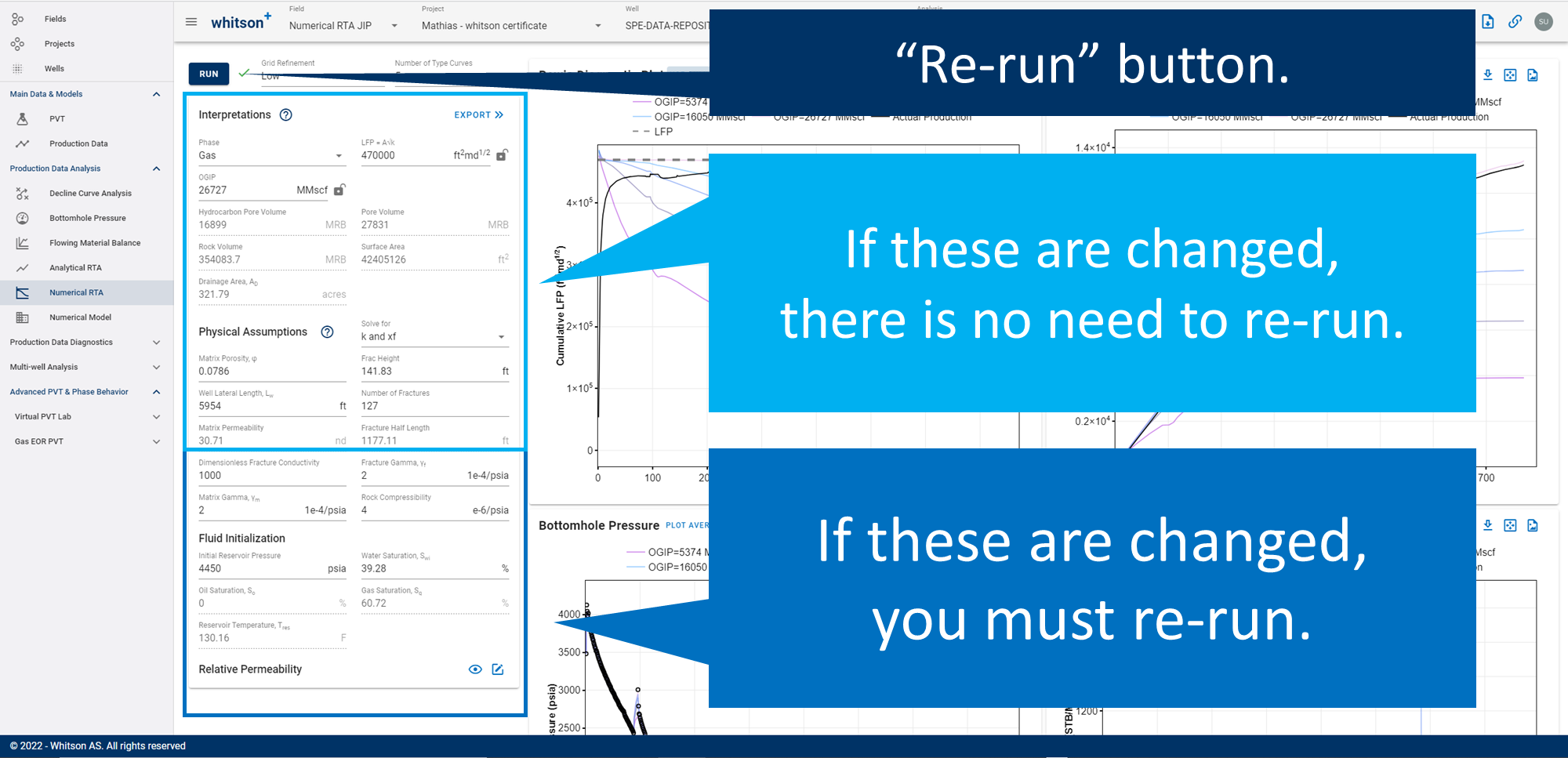
You will only need to re-run (click RUN) the numerical RTA module when you update any of the following parameters: PVT, S_wi, F_cd, relative permeability, pressure dependent permeability (gamma matrix/fracture) or initial pressure.

2.6.3 Numerical RTA - Second Run

You'll notice a bad match on the water cut. You can edit the Relative Permeability used to match water or gas cuts in the well. You can make modifications to this as follows -

You can create new relative permeability tables, or copy from your saved sets used previously. You also have the option to make these tables company wide.

Let's continue with the introduction, leave the relative permeability tables to default and not worry about matching water for this well!
However, the most likely realization should have convincing history matches in all the plots here.

Analytical LFP vs Numerical LFP

For gas wells that produce little water, you should expect the LFP in numerical RTA to be smaller than the one from analytical RTA. This is because analytical RTA only uses PVT properties at initial conditions to calculate LFP, while numerical RTA accounts for the changes in PVT properties due to changes in drawdown profile. Want to learn more? Contact support@whitson.com.

2.6.4 Numerical RTA - Export Results to Numerical Model

1. In the Numerical RTA module, click EXPORT in the top right of the Interpretation menu.
2. Read the pop-up box text and click YES.
3. The yellow exclamation mark indicates what has changed in the input compared to the previous simulation.
4. All steps are shown in the .gif above.

2.7 Numerical Model - History Matching

2.7.1 Well Control - Gas

1. In the Numerical Model module, click RUN in the upper left.
2. The first run of the numerical model should provide a very good history match.
   1. Your gas rates should be spot on (as you control the model on gas rate).
   2. Your bottomhole pressure fit should be great.
   3. Your water rate match could improve (we didn't do much here).
3. All steps are shown in the .gif above.

2.7.2 Well Control - Bottomhole pressure (BHP)

1. In the Numerical Model module, change the Well Control to BHP.
   1. This means we are controlling the model on bottomhole pressure.
2. Click RUN to the upper left, again.
3. This run should also be a very good history match, as none of the parameters have changed, only the well control. And this means:
   1. Your bottomhole pressure should be spot on (as you control the model on BHP).
   2. Your gas rate fit should be great.
   3. Your water rate match could improve (we didn't do much here).
4. All steps are shown in the .gif above.

2.7.3 Change Grid Refinement

1. In the Numerical Model module, change the Grid Refinement to Very Low.
2. Click RUN to the upper left, again. Notice any difference here?
3. All steps are shown in the .gif above.

2.7.4 Add a Forecast

1. Toggle the switch Include Forecast on.
2. Click the text Edit Forecast Schedule
3. Here, you can now forecast the wellhead pressure (WHP) or the bottomhole pressure (BHP)
4. Let's forecast the BHP - The Forecast type is Parametric Decline.
   1. Make the Forecast End Time 10 000 days (almost 30 years).
   2. Make the Final BHP 700 psia.
   3. Make the Nominal decline rate 2%/yr (notice that this can be adjusted to reflect a decline in BHP that you consider reasonable, based on the historical decline).
5. Click SAVE.
6. Click RUN to the upper left, again.
7. What is the gas EUR?
   1. If we assume Q_g at the end of 10 000 days (almost 30 years), somewhere around 21.5 bcf.
8. You can toggle 'Hide Forecast' to keep the forecast on the plots or remove them from view to see the history match without running again.
9. All steps are shown in the .gif above.

2.7.5 Remove the forecast

1. Toggle the switch Include Forecast off. This completely removes the forecast from the plots.
2. Click RUN to the upper left, again.
3. All steps are shown in the .gif above.

2.8 Numerical Model - Sensitivities

1. In the Numerical Model module, click the Sensitivities tab at the top left.

2. Ensure the well control says BHP.

   What is well control?

   The well control is what you are telling the numerical model is "known" while solving for all the other parameters. The numerical model will try to honor that input (e.g. gas rate) as long as the model is productive enough. For sensitivities and probabilistics, it can be useful to use BHP as the well control to ensure consistent results. Read more here

3. Open the input card named Sensitivities.

4. Select the parameters Matrix permeability and Fracture Half Length.
5. Click SAVE.
6. Click the MODIFY CASES button.
7. Fill in the case matrix below - you can set the line type and color for each of these cases if needed.
8. Click SAVE.
9. Click RUN to the upper left, again.
10. All steps are shown in the .gif above.

Case Matrix

When an input in the case matrix is left blank, it uses the default value for that input in that case.

Case #	Case Name	km	xf
1	Only perm	100
2	Only frac half-length		750
3	Both	10	1500

2.9 Numerical Model - Probabilistics

1. In the Numerical Model module, click the Probabilistics tab at the top left.
2. Ensure the well control says BHP.
3. Open the input card named Probabilistics.
4. Select the parameters Matrix permeability and Fracture Half Length.
5. Go to the tab named Case Overview.
6. Keep the number of cases 10 (or change to whatever you want).
7. Change the distribution type to normal distribution for both variables.
8. Keep the ranges as provided by default.
9. Click SAVE.
10. Click RUN to the upper left, again.
11. All steps are shown in the .gif above.

3. Black Oil ("Multiphase") Well

Wellname: SPE-DATA-REPOSITORY-DATASET-1-WELL-4-KITE

What if I get slightly different results than in these examples?

You might not get exactly the same results as the example below due to different EOS models. But no major difference is expected, regardless.

3.1 PVT

3.1.1 Reservoir Fluid Composition

1. Go to the PVT module in the navigation panel.
2. Open the Reservoir Fluid Composition Input Card
3. Initialize the fluid in the GOR method by moving the dashed horizontal line up and down to match the GOR calculated from the production data.
4. You can also input an initial GOR value in the box below. Enter 750 scf/STB.
5. Click SAVE.
6. Check the predicted fluid composition by clicking the "eye icon".
7. All steps are shown in the .gif above.

3.1.2 PVT Table

1. Go to the BLACK OIL TABLE tab.
2. Try to see if you can answer these questions yourself. No need to send these back to us, this is just for your own sake. You can reach out to support@whitson.com for a session to discuss this or send us a comment with your certification email if needed.
   1. What is the oil formation volume factor (B_o) and solution GOR (R_s)?
   2. Is this a saturated or undersaturated fluid system? What makes it so?
   3. Read up on the difference between total vs oil formation volume factor (B_t vs B_o) and total vs solution GOR (R_t vs R_o) (click here)
3. All steps are shown in the .gif above.

3.2 Production Data

In this section, we'll learn how to smooth production data.

3.2.1 Smoothing Production Data & Using Smoothed Data in Calculations

This example shows you how to smooth a timeseries in whitson⁺.

1. In the Production Data module, click SMOOTH up to the right, again.
2. Click AUTOFIT.
3. Change the Sampling Frequency from 20 to 10.
4. MOVE POINTS: Move one of the points somewhere else on the plot.
5. DELETE POINTS: Drag one of the points below 0 on the y-axis.
6. Make sure Oil Rate is checked under Use smoothed data to the left.
7. Click SAVE.
8. All steps are shown in the .gif above.

3.2.2 Smoothing Production Data - Reverting back to the Original / Unsmoothed Data

This example shows you how to deactivate the smoothing of timeseries data in whitson⁺.

1. In the Production Data module, click SMOOTH up to the right.
2. Uncheck the Oil Rate under Use smoothed data to the left.
3. Click SAVE.
4. All steps are shown in the .gif above.

3.3 Bottomhole Pressure

3.3.1 Calculate and Smooth Bottomhole Pressure

This example shows you how to calculate and smooth bottomhole pressures in whitson⁺.

1. Go to the Bottomhole Pressure module.
2. Click CALCULATE BOTTOMHOLE PRESSURE to the upper left.
3. Change the Bottomhole pressure to be used in calculations to Custom p_wf.
   If there is no Custom p_wf in the database, it automatically opens the 'Edit Custom BHP' dialog to create one. If you've already created a Custom p_wf for the well, you need to click 'Edit Custom BHP' button to open the editor.
4. In the 'Edit Custom BHP' window, click Autofit up to the left.
5. MOVE POINTS: Move one of the points somewhere else on the plot.
6. DELETE POINTS: Drag one of the points below 0 on the y-axis.
7. Click SAVE.
8. All steps are shown in the .gif above.

3.4 Flowing Material Balance (FMB)

3.4.1 Multiphase Flowing Material Balance

1. Go to the Flowing Material Balance module.
2. Click RUN to the upper left.
3. Try to write an OOIP number on the left. See how the slope is changing on the plot?
   Remember to hit Tab or Enter on your keyboard, or click outside of the input field, for it to update.
4. Now, zoom into the lower left portion of the data.
5. Fit a slope through the straight line portion of the data.
6. Write in 700 MSTB.
7. Click RUN one more time.
8. Ensure that the average pressure is higher than the bottomhole pressure in the plot up to the right.
9. All steps are shown in the .gif above.

Why do we zoom into the lower left of the data?

This is the portion of the data that with no free reservoir gas phase (bottomhole above saturation pressure). Hence, the compressibility of the system is lower, and seeing reservoir boundaries takes less time.

3.4.2 Recovery Factor Analysis

1. Click the tab named RECOVERY FACTOR ANALYSIS.
2. Graphically,

   Forecasting CGR and WGR vs pressure

   Follow the gif above to see how to add enough points and make a smooth forecast on the CGR and WGR plots for pressures down to 100 psia.
   

   1. Forecast the p_wf vs time plot.
3. Click RUN up the left.
4. Click the GOR VS. OIL button on the Instantaneous GOR plot to the top left. Does your forecast of GOR vs cumulative oil production look smooth/realistic?
5. What are the recovery factors? What are the predicted EURs? (Note these down for yourself, no need to send to us)
6. All steps are shown in the .gif above.

How to forecast CGR and WGR vs Pressure?

Regarding extrapolating OGR and WGR

R_v and 1/R_s curves are generated from the EoS based on the PVT initialization.

R_v or the condensate gas ratio represents the minimum oil that will be recovered at the surface as condensate dropout from gas production.
This represents the minimum oil evolved from gas that would still be recoverable when the oil phase stops being mobile and only gas is flowing. Hence, this volatilized Oil-Gas ratio, forms the minimum bound of the OGR expectation.

1/R_s or the oil gas ratio represents the maximum oil that has to be recovered to produce a unit volume of gas from solution. This essentially makes the upper bound of the ratio forecast.

Your forecasts will always be well within these bounds.

OGR data above the saturation pressure will be very close to the 1/Rs line and the forecast needs to follow the data and reasonably extrapolate to lower pressures (upto the abandonment pressure). Water Gas Ratio is typically declining with decline in pressure.

Reducing Uncertainty in Ratio Forecasting - See analogs!

In case the yield/GOR is a strong funciton of flowing bottomhole pressure - The case may not vary much with the type of analog chosen (parent/edge/fully bound), instead the analog must have similar producing history of sufficient length.

In case the yield/GOR is a strong function of average reservoir pressure - Split the data from analog wells by the type and select the trend that closely matches the type of the well, since parent wells will have a lowest, flat GOR while an edge and fully bound cases have different, but both sharply increasing trends in comparison. The forecast built should be bounded by the analog wells with the fully bounded tight infill yields the sharpest increase in GOR while the parent well offers a minimum bound for the magnitude and the rate of change of GOR.

Finally, always use the Cumulative GOR vs Cumulative Oil to sanity check the forecast - realistically, you expect a linear increase with a concave up trend.

Impact of these forecasts on recovery factors

The oil EUR and recovery factors are far less sensitive and gas EUR may be slightly more sensitive to the constructed forecast in WGR.
The most practical uncertainty you might face is the OGR ratio forecasting, which also has the highest impact on calculated recovery rates.

MFMB vs Numerical Model recovery factors

In MFMB, we forecast the ratios and use simple material balance equations to calculate Recovery Factors and EUR. We proceed in the opposite direction compared to the Numerical Simulations, where we run a numerical simulation to get the same ratios over time to ultimately calculate the Recovery factors and EUR.

Under the assumption that most unconventional wells produce from reservoirs with an expansion-drive, if the forecasted ratios and abandonment pressures are exactly the same in Numerical Model and MFMB, we get the exact same recovery factors and EUR as well.

Why are the recovery factors so high?

These recovery factors are recovery factors of the contacted pore volume. The contacted pore volume, sometimes called the stimulated rock volume (SRV) or the drained rock volume, is the volume resolved from RTA. It is NOT the petrophysically mapped pore volume, which typically is 2-5 times as large as the contacted pore volume. Hence, the recovery factors of the petrophysical pore volume is 2-5 times less than these recovery factors (typically below 10%). Want to learn more? Contact support@whitson.com.

3.5 Analytical RTA

3.5.1 Classical RTA

1. Go to the Analytical RTA module.
2. Click AUTOFIT up to the left.
3. If you want to, change the slope in the Square Root of Time plot.
   1. This is the upper left of the four plots on the screen.
   2. Go to the end of the slope until the cursor icon changes to a hand.
   3. Click and drag to match the slope of the data.
   4. A shallower slope --> increases the A√k (also called the Linear Flow Parameter - LFP)
   5. A steeper slope --> decreases the A√k
4. If you want to, move the dashed vertical line to change time to end of linear flow (t_elf).
   1. A higher time to end of linear flow --> higher OOIP
   2. A lower time to end of linear flow --> lower OOIP
5. All steps are shown in the .gif above.

3.5.2 Fractional RTA

1. Click the tab named Fractional RTA.
2. Change the delta (𝛿) parameter to 0.5.
3. Move the slope across the part of the data that fits a delta (𝛿) of 0.5.
4. Change the delta (𝛿) parameter to 0.
5. Move the slope across the part of the data that fits a delta (𝛿) of 0.
6. What flow regime do you think the well is in at the end of history? (write this down for yourself, no need to send to us, but you can send it together with the certification email if you would like our feedback)
7. All steps are shown in the .gif above.

What is the physical significance of 𝛿?

In material balance time,
𝛿 = 0.5 --> infinite acting (IA) flow
0 < 𝛿 < 0.5 --> transitional flow
𝛿 = 0 --> boundary dominated flow (BDF)

3.6 Numerical RTA

3.6.1 First run...

1. Go to the Numerical RTA module.
2. Click RUN.
3. Before picking a LFP=A√k and OOIP, first things to check:
   1. Check your producing water cut match. Is the model under- or overpredicting history? This plot is the one in the lower left, the model is in the different shades of blue / purple while the history is in black.
   2. Check your producing GOR match. Are you under- or overpredicted? This plot is the one in the upper right, , the model is in the different shades of blue / purple while the history is in black.
   3. Before picking an LFP & OOIP, the first thing we need to do is to decently match stabilized water cuts and GORs.
4. All steps are shown in the .gif above.

3.6.2 Second run...

1. Adjust the relative permeabilities
   1. S_wc = 20 -> S_wc = 0 (will increase water cut).
   2. S_gc = 5 -> S_gc = 0 (will make GOR increase earlier in time).
2. Click RUN, again.
3. Change the LFP=A√k value to 60 000 ft²md^1/2.
4. What OOIP is automatically picked by the software?
   1. whitson⁺ automatically picks the stem that is closest to the data at end of history.
   2. The OOIP should be close to 840 MSTB.
5. Double-click the OOIP in the legend that is closest to your observed data, or CTRL+click on the curve in the plot.
   1. Now only two curves should show in the plot; the actual production data and your pick of OOIP stem.
6. All steps are shown in the .gif above.

Oil wells: Analytical LFP vs Numerical LFP

For oil wells that produce water, you should expect the LFP in numerical RTA to be larger than the one from analytical RTA. This is because numerical RTA accounts for multiple phases flowing in the reservoir (o + g + w), while analytical RTA accounts for one phase (when Phase is set to 'oil').

3.6.3 Export to Numerical Model

1. Click EXPORT on the top left.
2. Click yes in the pop-up.
3. All steps are shown in the .gif above.

3.7 Numerical Model

3.7.1 History Matching

1. In the Numerical Model module, click RUN in the upper left.
2. Your first run should provide a very good history match.
   1. Your gas rates should be spot on (as you control the model on gas rate).
   2. Your oil rates should be great.
   3. Your bottomhole pressure fit should be great.
   4. Your water rate fit should be decent (we didn't do much here).
3. All steps are shown in the .gif above.

3.7.2 History Matching - Forecast

1. Toggle the switch Include Forecast on.
2. Click the text Edit Forecast Schedule
3. Here, you can now forecast the wellhead pressure (WHP) or the bottomhole pressure (BHP)
4. Let's forecast the BHP - The Forecast Type is Parametric Decline.
   1. Make the Forecast End Time 10 000 days (almost 30 years).
   2. Make the Final BHP 700 psia.
   3. Make the Nominal decline rate 10%/yr.
5. Click SAVE.
6. Click RUN to the upper left, again.
7. What is the oil EUR?
   1. If we assume Q_o at the end of 10 000 days (almost 30 years), somewhere around 170 MSTB.
8. All steps are shown in the .gif above.

3.8 Analyses

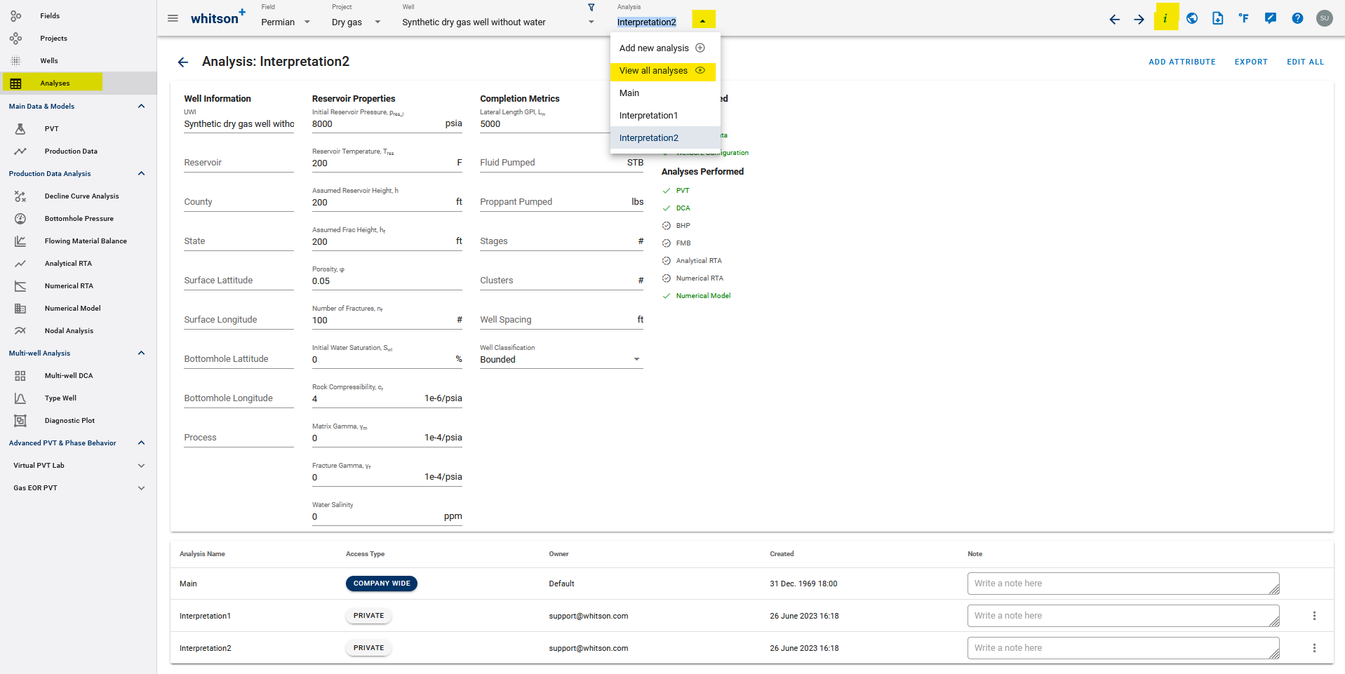
3.8.1 Save an Interpretation

1. Click the Analyses drop down menu in the Top Bar (next to well name).
2. Click Add New Analysis.
3. Provide a proper name and click YES.
4. The previous case you worked on has now been saved, and you can change any of your interpretations (PVT, BHP, FMB, RTA, etc.) without changing the other analyses.
5. The only thing that is the same for the different analyses is the raw production data.
6. All calculations can be different for the different analyses if you want to (PVT, BHP, FMB, RTA, numerical model). So, for example one can try a new analysis with lower Fcd, or a different reservoir pressure.
7. All steps are shown in the .gif above.

3.8.2 Navigating through Analyses

• You can click the 'Analyses' button on the navigation pane on the left, below 'Wells'.
• You can also use the dropdown menu on the Top Bar under 'Analyses' to create a new analysis, switch to different analyses or view them all.
• You can also click the 'i' icon at the top-right to the page to view the main well overview page to view all analyses.

P.S. Hovering over the 'i' icon can also show key results from different features for comparisons.

Three main ways highlighted below.

4. Sharing your Project

Projects and individual analyses within wells have the following privacy options -

1. Company-wide - Everyone in the company will be able to see and modify the project/analysis by simply navigating to it on whitson⁺.
2. Private - Visible only to you/owner unless a link is shared. Then, clicking the link and logging in allows access to the recipient of the link only.

How to share a project or analysis using a link?
Simply copy the URL link on the browser window and send it across. Done!

5. Do it yourself

5.1 Perform a workflow yourself

Wellname: SPE-DATA-REPOSITORY-DATASET-1-WELL-10-CROW

Perform the following workflow on the last well, including

1. PVT
2. Bottomhole pressure calculation (BHP)
3. Flowing Material Balance (FMB) & Recovery Factor (RF) Analysis
   1. Final Pressure = 500 psia for RF analysis
4. Analytical RTA (both classical and fractional)
5. Numerical RTA
6. Numerical Model (with a forecast)
   1. Final Pressure = 500 psia (use parametric decline)
   2. Total simulation time = 10 000 days

5.2 Done?

When you are done with your interpretation of this last well Wellname: SPE-DATA-REPOSITORY-DATASET-1-WELL-10-CROW, please:

1. Send an e-mail to certification@whitson.com
2. Make the subject: "whitson⁺ certificate: [YOUR NAME HERE]".
3. Include the link to your project.
4. Report the following from the Flowing Material Balance and Recovery Factor Analysis feature for this last well that you did on your own.
   1. Contacted OOIP & OGIP
   2. EUR from gas and oil
5. Report the following from the Numerical model for this last well that you did on your own.
   1. Contacted OOIP & OGIP
   2. EUR from gas and oil
6. If you have any notes, comments, or observations related to the well, feel free to share them with us. Also feedback on the user friendliness of the software is always appreciated.

After that we'll provide some feedback on your evaluation and issue your whitson⁺ certificate if all looks good.