whitson⁺ - Auto-Forecast & Type Well Certification

1. Introduction

Complete the steps outlined below to become an DCA & Type Well certified whitson⁺ user. It includes performing auto-forecast and type well creation. Those certified have the software skills necessary to complete most type well evaluation projects in tight unconventionals.

Need help?

Send an email to support@whitson.com.

1.1. Before Starting

Make sure you watch the following three introductory videos in the Getting Started section of manual:

• Login (1 min)
• Overview of important basics (3 min 30 sec)
• Zooming and navigating plots (3 min)

1.2. Create a Project

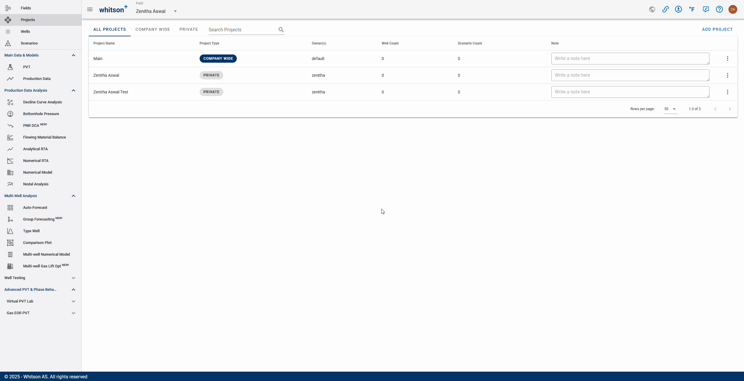
1. Go to the Projects module from the navigation panel.
2. Click ADD PROJECT in the upper-right corner.
3. Enter the project name as "Your Name - whitson Certificate - Type Well".
4. Click SAVE to create the project.
5. The full process is illustrated in the GIF above.

1.3. Upload the Data

1. Click MASS UPLOAD in the upper-right corner.
2. In the pop-up window, select EXAMPLES
3. Search for Auto-Forecast & Type Well Certificate Wells, then click UPLOAD
4. Wait for the data to be uploaded to the project.
5. Once the upload is complete, close the Mass Upload pop-up window.

The complete step is illustrated in the GIF above.

2. Auto-Forecast

2.1. Create an Auto-Forecast

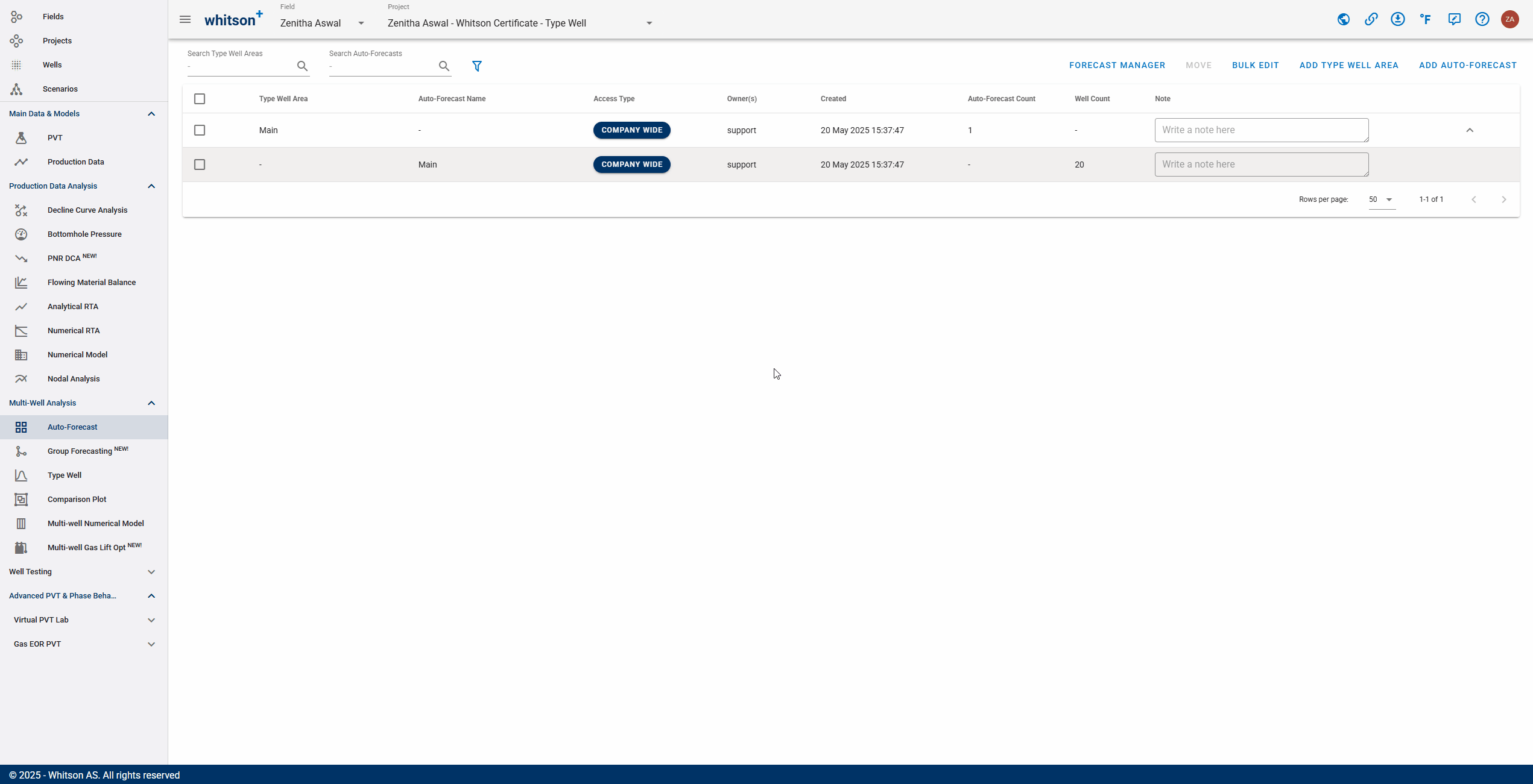
1. Select Auto-Forecast module from the navigation panel.
2. Click ADD AUTO-FORECAST in the upper-right corner.
3. Enter a name for the Auto-Forecast.
4. Select all wells by clicking the checkbox at the top of the well list, to the left of Well Name.
5. Click ADD AUTO-FORECAST in the lower-left window.

You can store multiple auto-forecasts in a project

This page overview displays all Auto-Forecasts created in the project, including when each Auto-Forecast was created, who created it, and which wells were included.

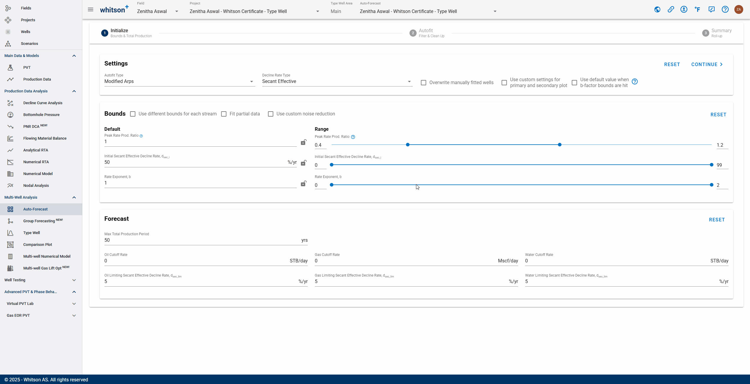
2.2. Initialize the Auto-Forecast

The GIF below shows the settings and functionality available when initializing an Auto-Forecast.

Related DCA Settings

For more information about Autofit Type and the available segment types, see Other Segment Types.

For more information about Decline Rate Type, see Effective Decline.

Initialize the Auto-Forecast using the parameter ranges shown below.

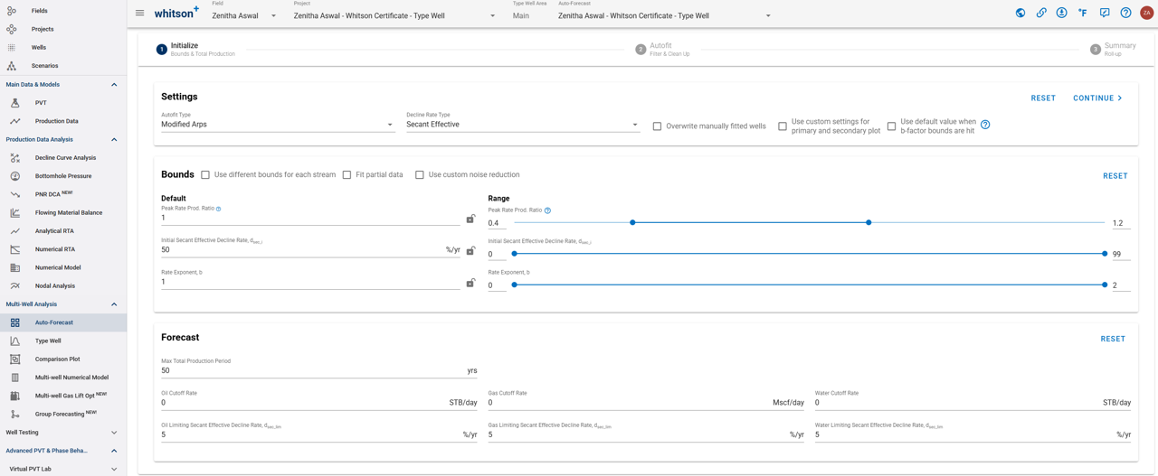
What is the Peak Rate Production Ratio?

The Peak Rate Production Ratio constrains the range of $q_i$ values that can be fitted by the DCA model. The range is defined as a fraction of the historical peak production rate.

For example, assume that the maximum historical oil rate for a well is 1,000 STB/d. A Peak Rate Production Ratio ranging from 0.8 to 1.2 allows the fitted $q_i$ to range from: $$0.8 \times 1{,}000 = 800\ \text{STB/d}$$ to: $$1.2 \times 1{,}000 = 1{,}200\ \text{STB/d}$$ This provides a general method for defining appropriate $q_i$ ranges across multiple wells and production streams, including oil, gas, and water.

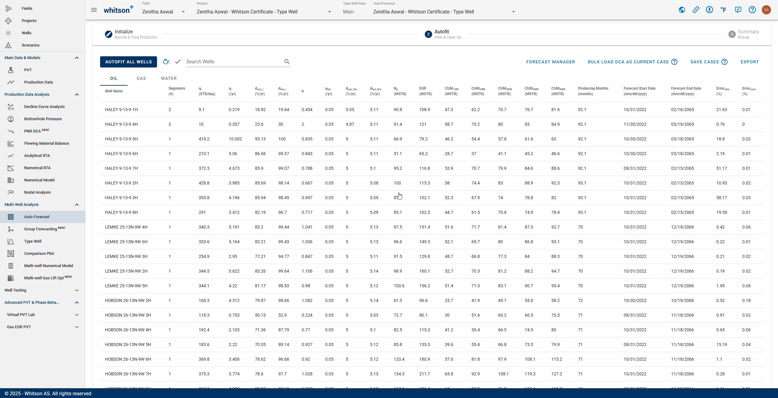
2.3. Autofit All Wells

1. Click CONTINUE in the upper-right corner, or select the second step in the tab 2 Autofit.
2. Click AUTOFIT ALL WELLS in the upper-left corner.
3. Review the fitting summary for each production stream by selecting the OIL, GAS, or WATER tab.

How does the default autofit work?

For each production stream, the autofit first identifies the time step associated with the historical peak rate. It then estimates the DCA parameters within the ranges defined during initialization and selects the parameter combination that provides the best fit to the production history.

2.4. Sort the Auto-Forecast Summary

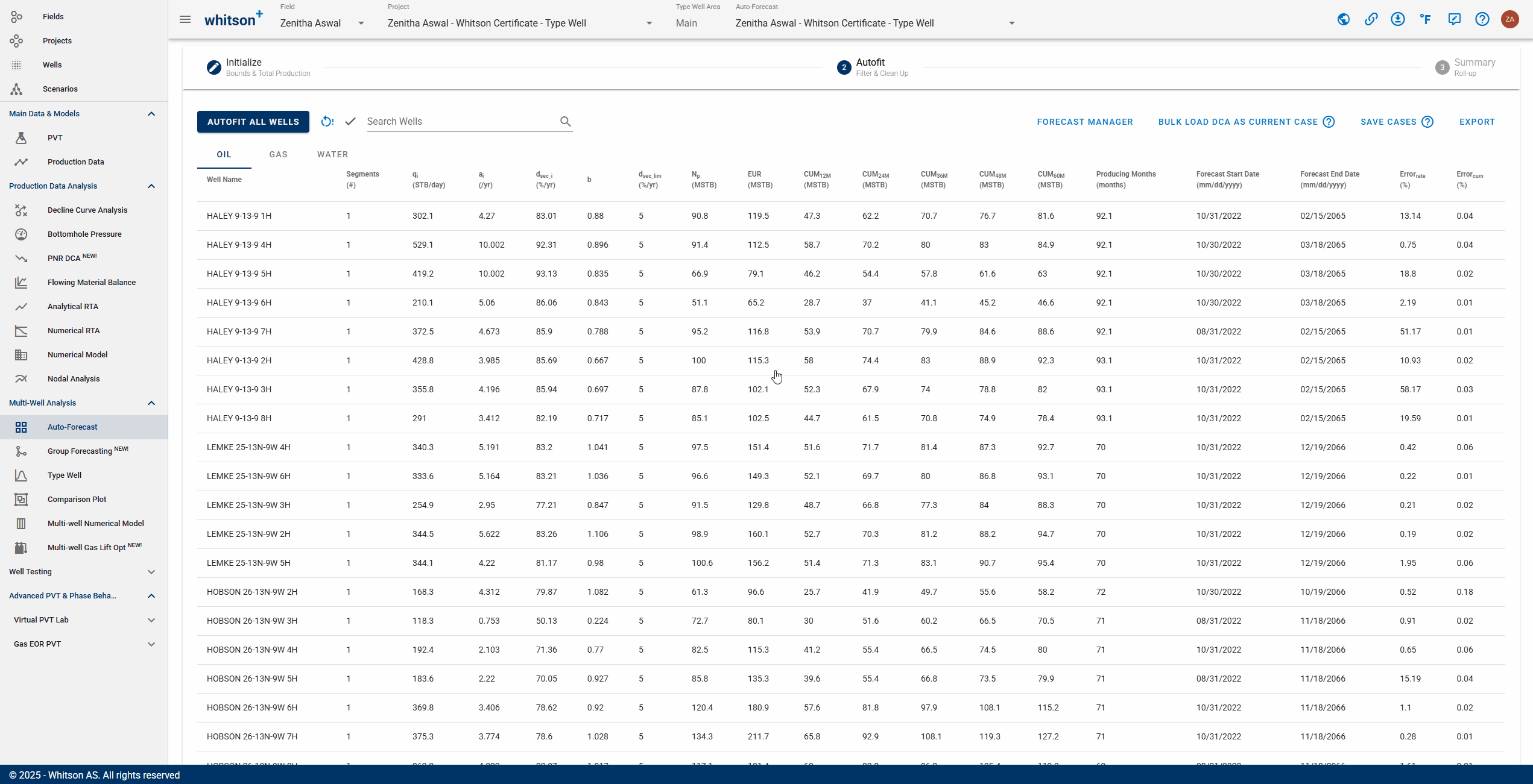
You can sort the wells by clicking any column header in the Auto-Forecast summary table.

For example, click the $b$-factor column header to sort the table by $b$-factor:

• Click once to sort from minimum to maximum in ascending order.
• Click again to sort from maximum to minimum in descending order.
• Click a third time to return to the original, unsorted order.

Why should I sort the results?

When working with many wells, sorting helps identify fits that may require additional review. For example, you can sort the table by fitting error and manually inspect only the wells with the largest errors.

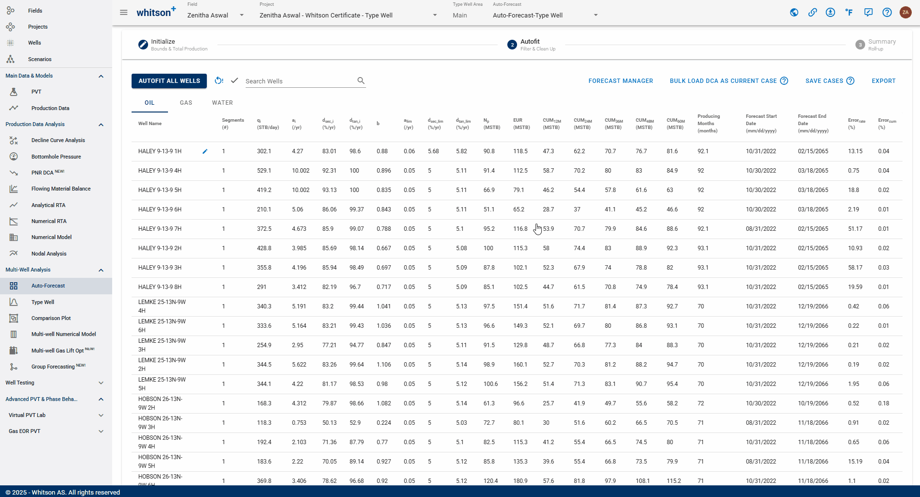
2.5. Manually Review the DCA Fits

You can manually review and adjust the DCA fit for each well from the Auto-Forecast summary table.

1. Click a well row in the table. A window displaying the single-well DCA fit will open.
2. Use the right arrow (→) in the upper-right corner of the DCA Fit window to move to the next well.
3. Use the left arrow (←) to return to the previous well.

You can also use the following keyboard shortcuts:

• Press Page Down to move to the next well.
• Press Page Up to return to the previous well.

What does the DCA $b$-factor represent?

The DCA $b$-factor controls the curvature of the decline trend and describes how the effective decline rate changes as production decreases. A lower $b$-factor generally produces a more rapid transition toward exponential decline, while a higher $b$-factor produces a longer and more gradually declining production tail. The $b$-factor may be related to reservoir flow behavior when the fit is performed under relatively stable operating conditions, particularly when flowing bottomhole pressure is approximately constant. However, it should not be interpreted as a standalone measurement of recovery efficiency.

2.6. Manually Adjust the DCA Fit

The DCA fit can be adjusted in two ways:

1. Enter the desired parameter values directly in the input fields.
2. Adjust the fit graphically by moving the available control points on the plot.

The GIF above illustrates an example of manually adjusting a DCA segment.

You can add multiple decline segments

Using multiple DCA segments can provide a better representation of actual production behavior, particularly when a well transitions between different flow regimes. A single decline segment may not capture these changes and can result in an oversimplified forecast. Learn more about adding multiple decline segments.

2.7. Save the Cases

1. Click SAVE CASES in the upper-right corner.
2. Enter Base Case as the DCA forecast name.
3. Save the case.

This creates a saved DCA case for each well and each production stream included in the Auto-Forecast.

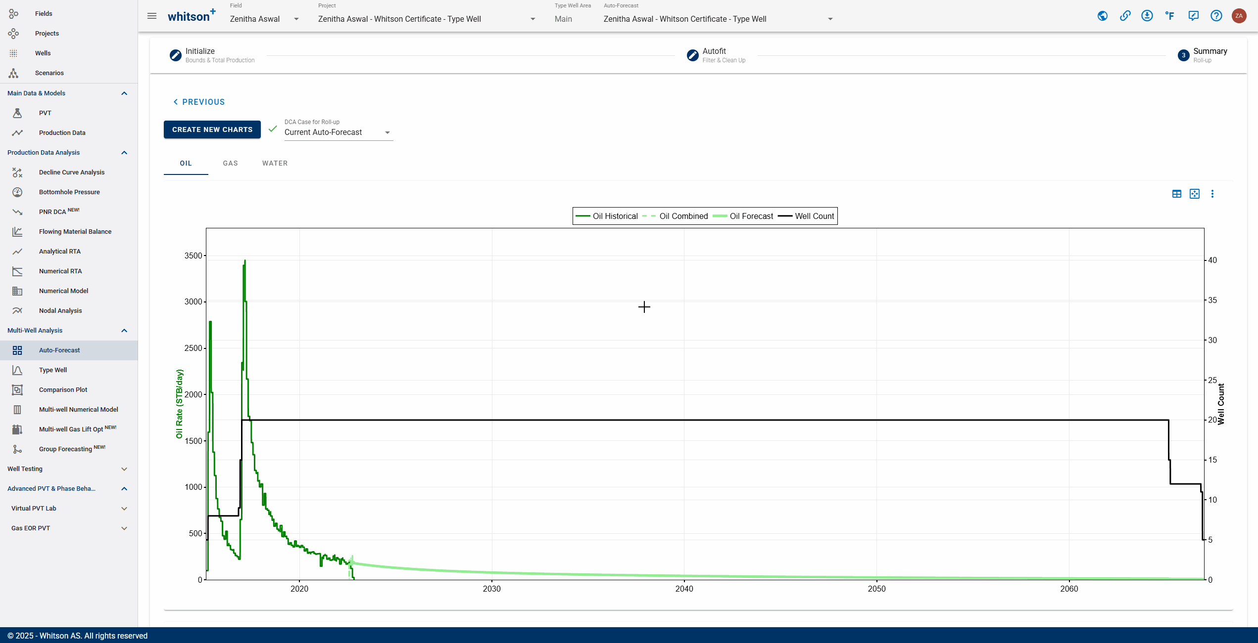
2.8. Perform a Roll-up

A roll-up can be used to quality-check the overall Auto-Forecast results. The roll-up combines the production rates from all selected wells at each time step and displays the aggregated results in both rate and cumulative space.

Review the resulting plots to confirm that the transition from historical production to forecasted production is smooth and does not contain unexpected discontinuities.

To create a roll-up:

1. Go to the Forecast Manager module from the navigation panel.
2. From the Selected Forecast drop-down menu in the upper-left corner, select Base Case.
3. Select the phase or production stream you want to display using the option below the Selected Forecast drop-down menu.
4. After selecting the desired stream, click ACTIONS in the upper-right corner.
5. Select Rollup from the menu.

What should I check in the roll-up?

Pay particular attention to the transition between historical and forecasted production. Sudden increases, decreases, or discontinuities may indicate that one or more individual-well forecasts should be reviewed.

2.9. Return to the Auto-Forecast Overview

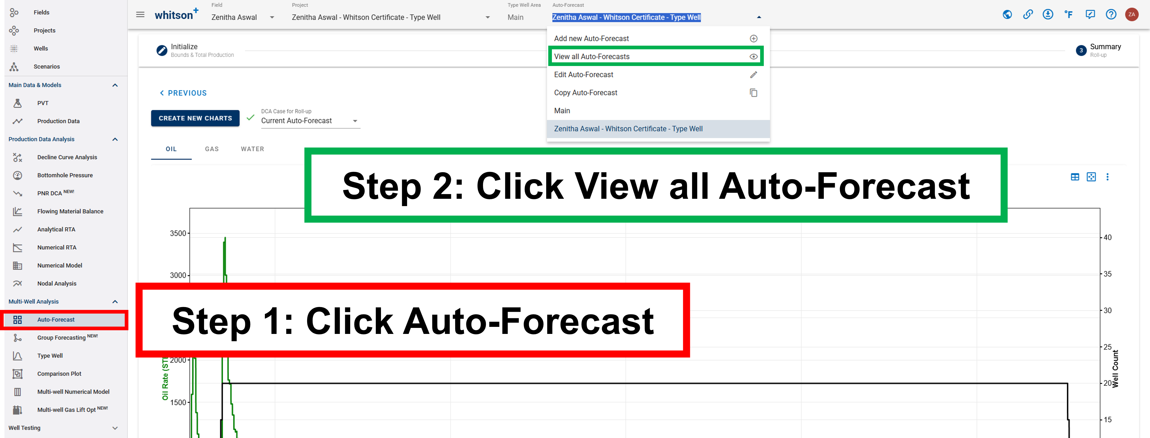
You can return to the Auto-Forecast overview using either of the following methods:

1. Select Auto-Forecast module from the navigation panel.
2. Click the current Auto-Forecast dropdown in the top menu bar and select View all Auto-Forecasts.

2.10. Edit the Auto-Forecast Well Selection

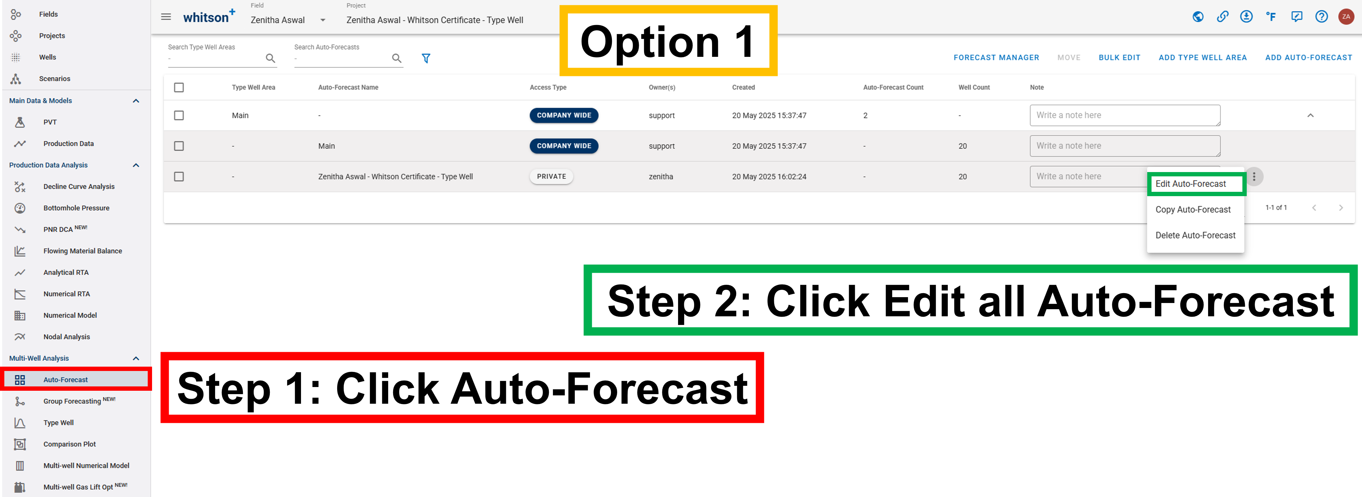
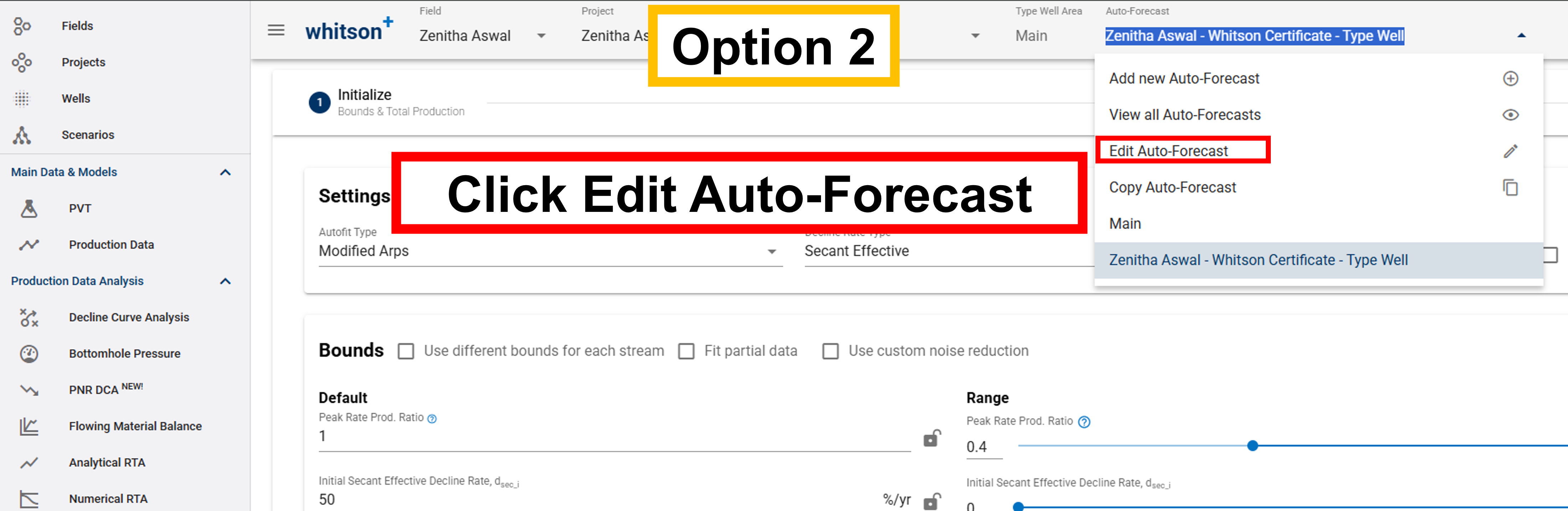
You can edit the wells included in an existing Auto-Forecast using either of the following methods:

1. Open the Auto-Forecast Overview, then select Edit Auto-Forecast.
2. Click the current Auto-Forecast dropdown in the top menu bar and select Edit Auto-Forecast.

After updating the well selection, save the changes before continuing.

3. Type Well

A type well represents a typical production profile for a group of analogous wells over a specified period.

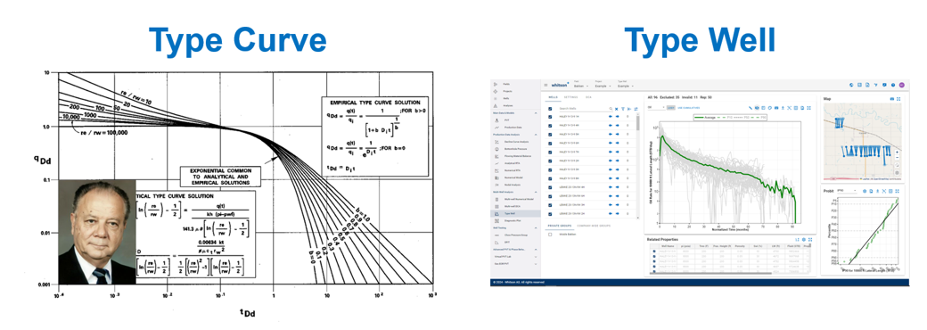
Although the terms type well and type curve are sometimes incorrectly used interchangeably, they have different meanings:

• A type curve is typically an idealized production profile generated from analytical equations, numerical simulation, or another modeling approach.
• A type well is generated from actual well-production data and represents the expected or typical production profile of a selected group of wells.

What is a typical well?

An arithmetic mean is commonly used to estimate the representative production profile of a group of wells. However, when production rates and EURs follow an approximately lognormal distribution, the geometric mean may better represent the central tendency and be less sensitive to high-value outliers. whitson⁺ calculates both arithmetic and geometric means, allowing you to compare the two methods and select the most appropriate representation for your dataset.

3.1. Create a Type Well

1. Select Type Well module from the navigation panel, directly below Auto-Forecast module.
2. Click ADD TYPE WELL PROJECT in the upper-right corner.
3. Enter a name for the type well "Your Name - whitson Certificate - Type Well"..
4. Select all wells by clicking the checkbox at the top of the well list, to the left of Well Name.
5. Click ADD TYPE WELL in the lower-right corner.

You can store multiple type wells in a project

The Type Well overview displays all type wells created in the project, including when each type well was created, who created it, and which wells were included.

3.2. Select Wells

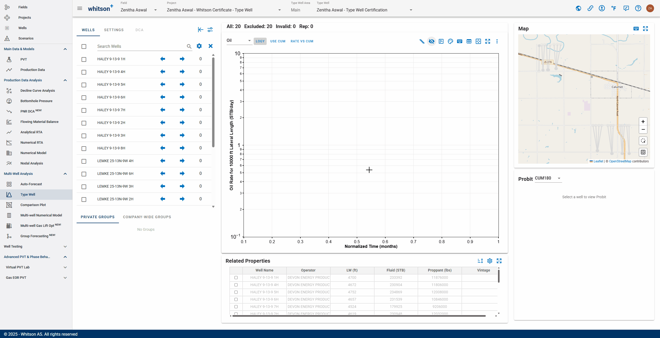
Use the checkboxes in the well list to select the wells included in the type well.

You can use the search field or map to locate specific wells before selecting or clearing them.

3.3. Normalization

Normalization places wells on a consistent basis so that their production profiles can be meaningfully compared and averaged.

The Type Well workflow supports time alignment, time-axis selection, and dimensional normalization.

3.3.1. Start Time Alignment

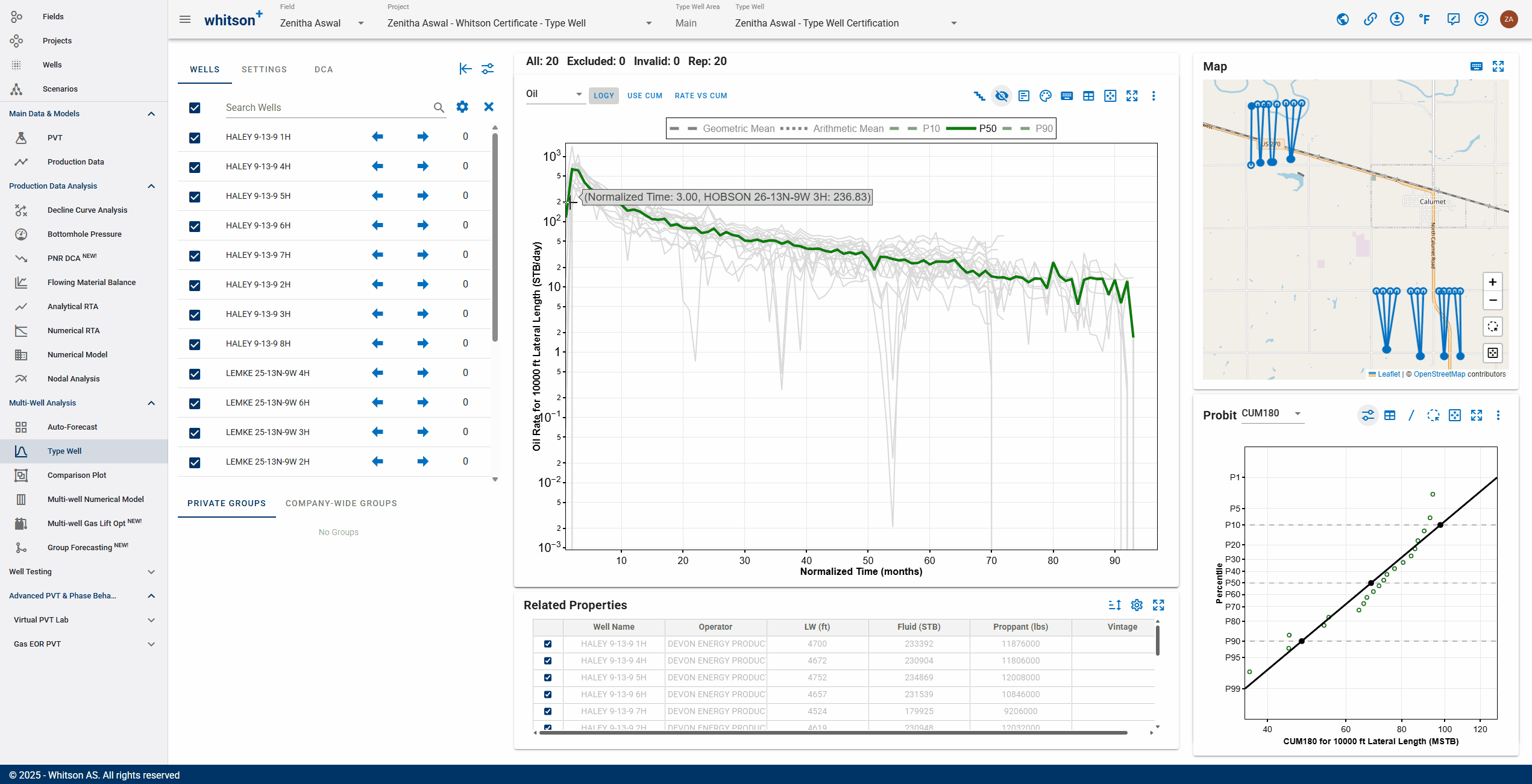
For this example, align the wells at the peak production rate, as illustrated in the GIF above.

Time-alignment options

Align on First Production

• Strength: includes the ramp-up period and time to peak, which may be important when estimating early-time production and first-year revenue.
• Limitation: differences in startup operations may obscure the underlying decline behavior.

Align on Peak Rate

• Strength: aligns wells at a comparable production milestone and generally provides a clearer comparison of decline behavior.
• Limitation: excludes the pre-peak ramp-up period, which may have a small effect on EUR but can affect early-time production and revenue estimates.

3.3.2. Condensing Time

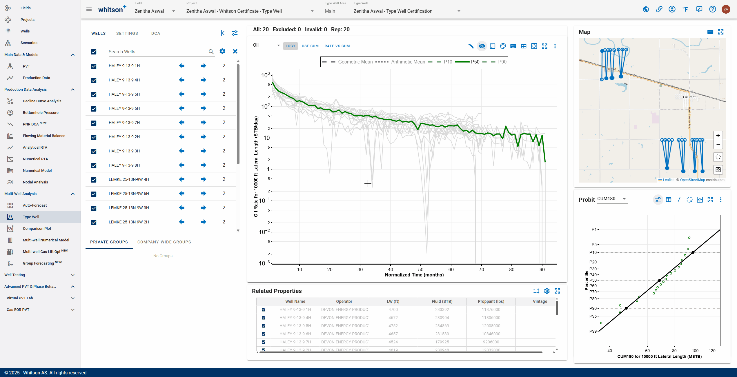
1. Click the SETTINGS tab in the upper-left corner.
2. Open the X Axis drop-down menu.
3. Select Normalized Flowing Time (by stream).

For this example, keep the default Normalized Flowing Time (by stream) setting. Review the available options below to understand how each time axis treats non-producing periods.

Available x-axis options

1. Normalized Flowing Time (by stream): includes only time steps where the selected stream—oil, gas, or water—has a nonzero production rate.
2. Normalized Flowing Time (by total production): includes only time steps with active oil, gas, or water production. Time steps where all production rates are zero are excluded.
3. Normalized Time: aligns the time axis based on the selected start-time alignment.
4. Cumulative Production: displays cumulative production on the x-axis instead of time.

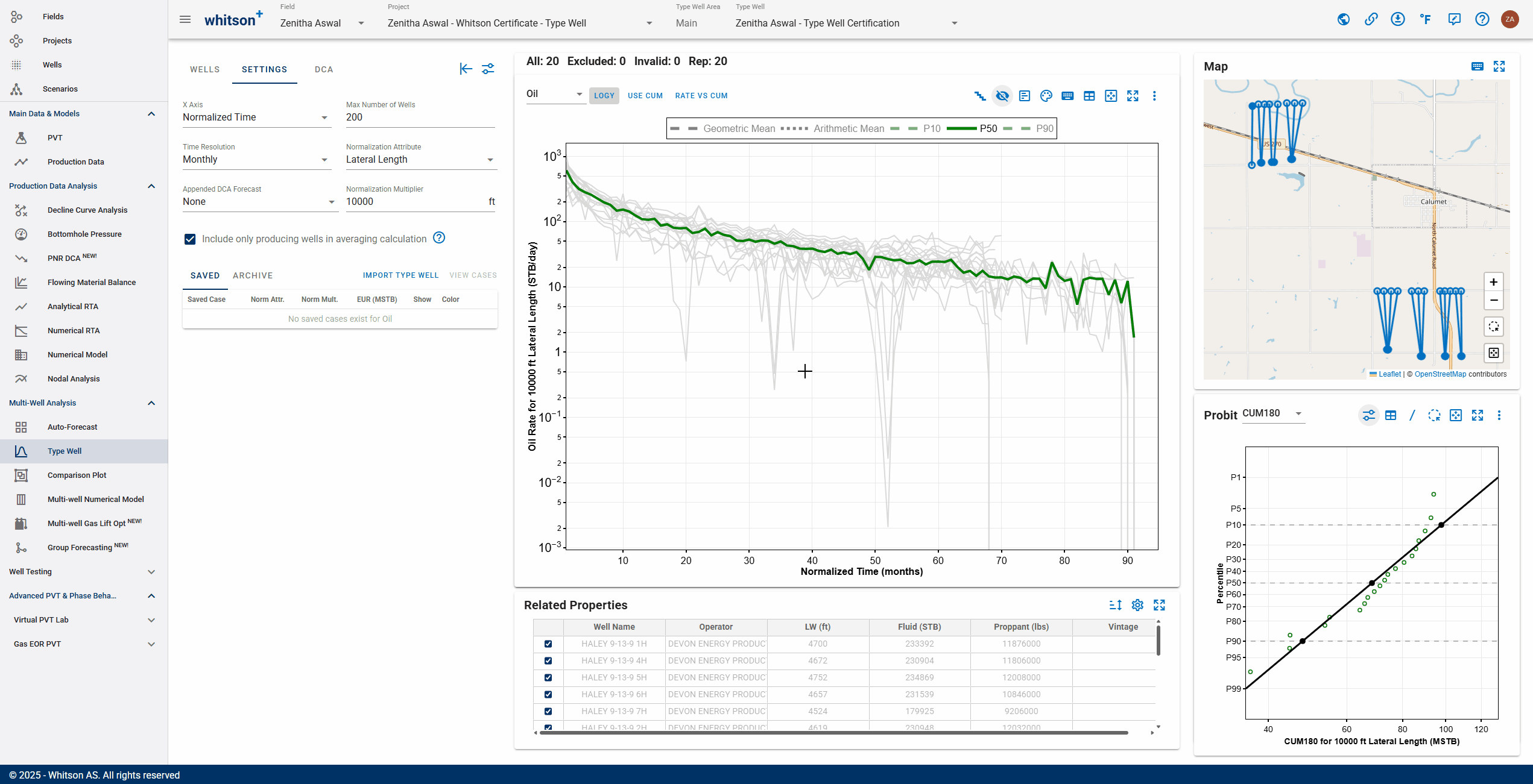
3.3.3. Dimensional Normalization

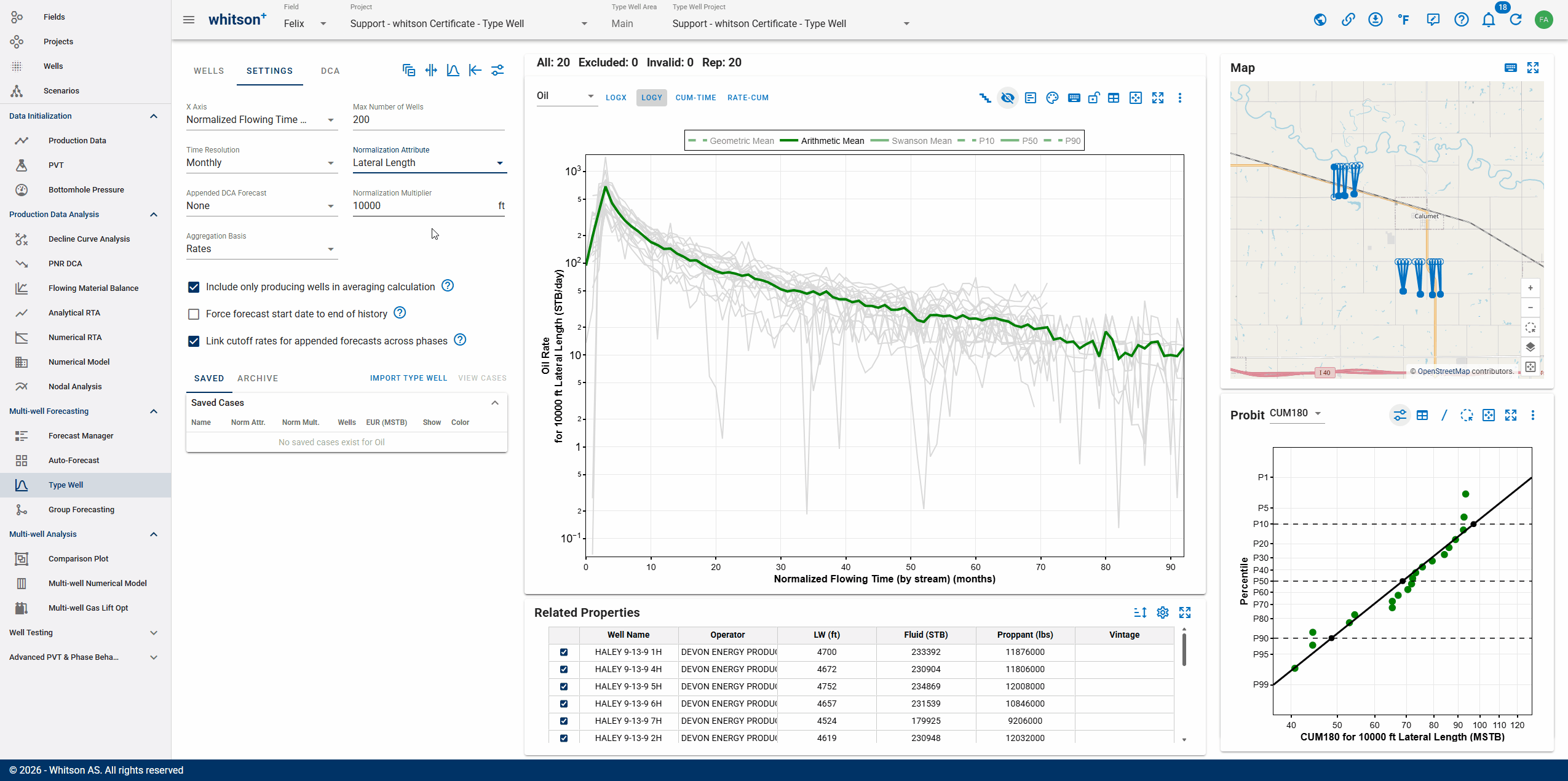
Dimensional normalization places wells with different physical dimensions on a comparable basis.

A common approach is to normalize production by lateral length. In this example, production will be normalized to a 10,000-ft lateral.

By default, new type wells are normalized by lateral length using a multiplier of 10,000.

Nonlinear normalization

whitson⁺ also supports nonlinear normalization. This method is not covered in this certificate workflow. For more details, navigate to Type Well manual.

3.4. Averaging Method

The Type Well module provides four three averaging methods:

1. Geometric Mean

   The geometric mean is calculated by multiplying the positive values and taking the (n)-th root, where (n) is the number of contributing values. It can provide a more representative central tendency for approximately lognormal datasets and is generally less influenced by high-value outliers.

2. Arithmetic Mean

   The arithmetic mean is calculated by summing the values from the selected wells at each point and dividing by the number of contributing wells.

3. Swanson Mean

   The swanson mean approximates the expected value of a probability distribution using the P10, P50, and P90 values: 0.3 P90 + 0.4 P50 + 0.3 P10

By default, the plot will show Arithmetic Mean. Other series may initially be hidden on the plot. Select the corresponding series to display them.

For this exercise, use the P50 as the base for fitting DCA segment to the type well profile.

Geometric Mean

“The geometric mean better approximates the median. Medians are more predictive for the outcome of a small number of samples—in this case, drilled wells—as well as being much more robust to outliers. Since production rates and EURs are generally distributed lognormal, an average of the logs of values makes a lot of intuitive sense.”

— David Fulford

3.5. Overview of Plot Options

Watch the video above for an overview of the available Type Well plot options.

3.6. Forecast the Average vs. Average the Forecasts

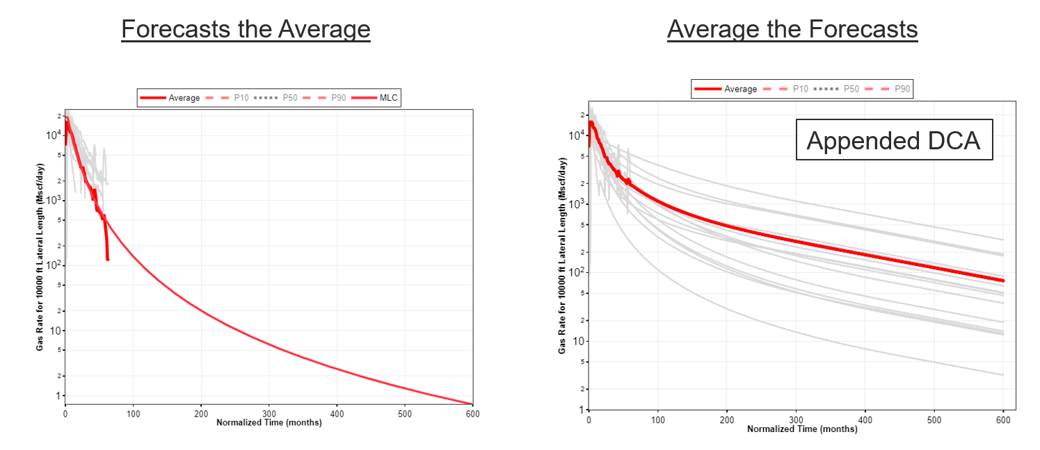
There are two approaches for incorporating forecasts into a type well:

• Forecast the Average
• Average the Forecasts

In this example, the saved individual-well forecasts from the Auto-Forecast workflow will be appended before calculating the type well.

3.6.1. What Is the Difference?

Forecast the Average

• First calculates the average historical production profile.
• Applies a DCA forecast to the resulting average profile.
• Provides a quick and efficient method for generating a full-life production profile.
• Does not preserve the distribution of individual-well EURs.

Average the Forecasts

• First generates or appends a forecast for each individual well.
• Calculates the average from the complete historical-plus-forecast profiles.
• Preserves the distribution of individual-well results.
• Supports statistical evaluation of metrics such as EUR and P10/P50/P90 estimates.

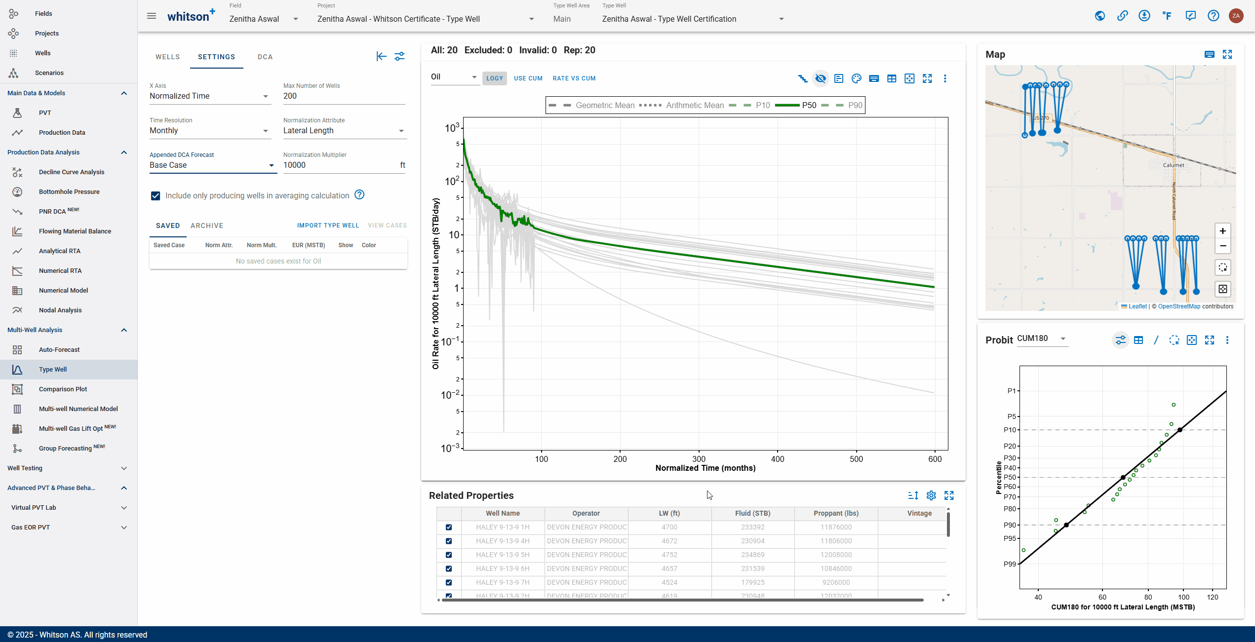
3.6.2. Append a DCA Forecast

Append the saved DCA "Base Case" forecast generated during the Auto-Forecast workflow, as illustrated in the GIF above.

For more information about the difference between cumulative calculations in Type Well and DCA, see Cumulative Calculation in Type Well vs. DCA

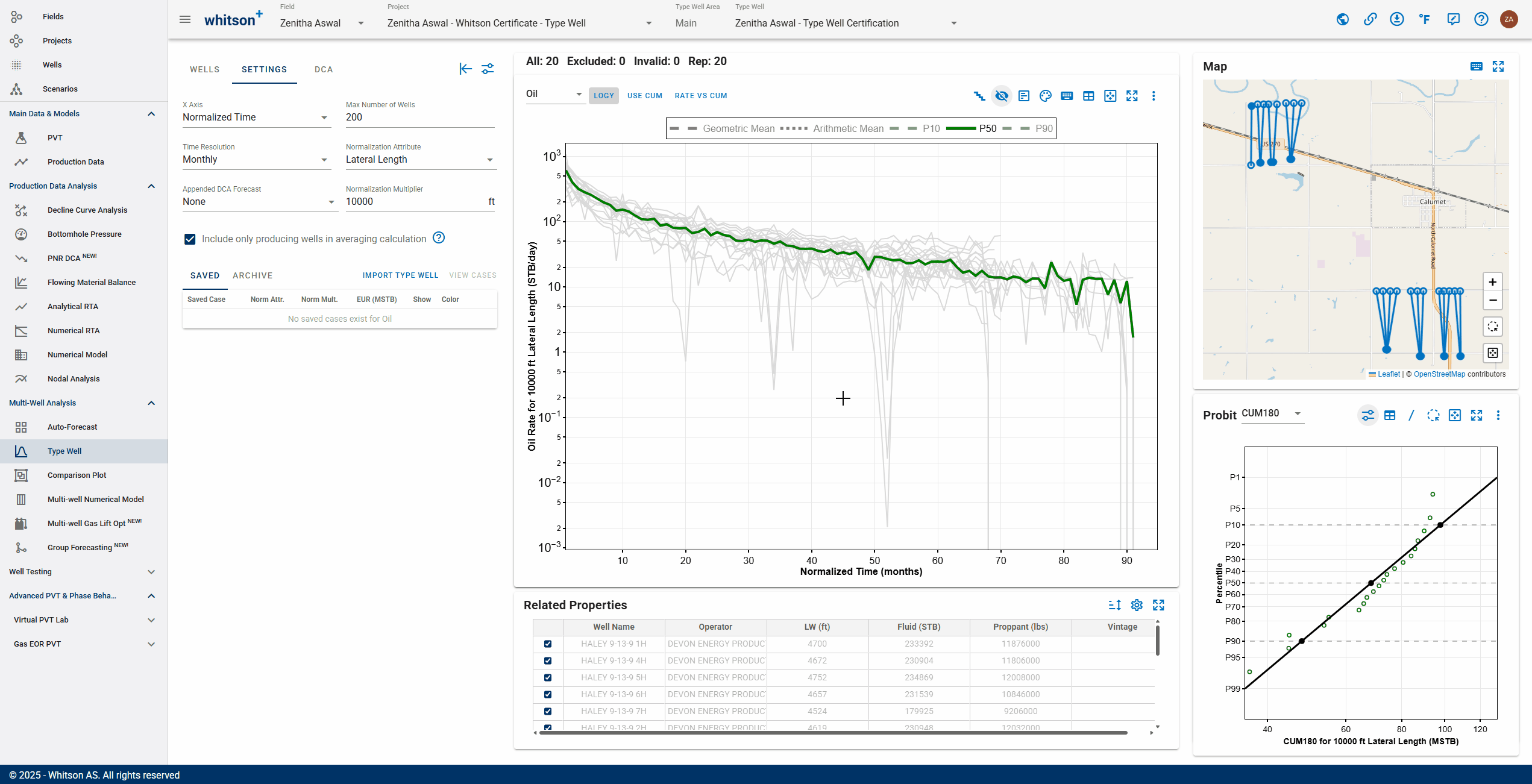
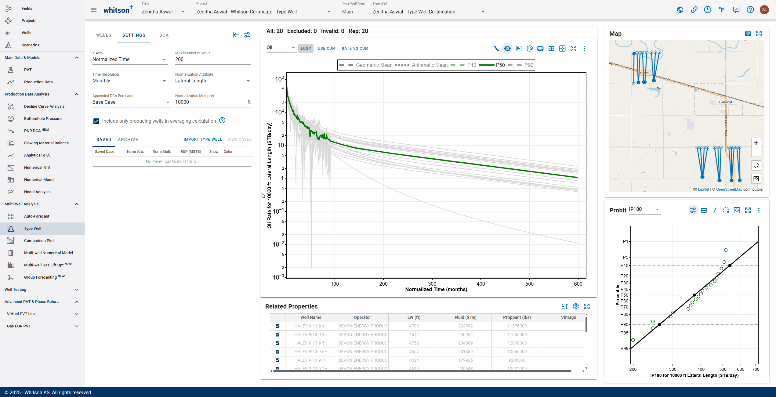
3.7. Probit Plot

A probit plot displays the statistical distribution of a selected property, such as EUR, IP60, or a physical well parameter.

The plot can be used to:

• Evaluate the distribution of results at a selected time or production point.
• Assess whether the data approximately follow a lognormal distribution.
• Identify potential outliers or separate well populations.
• Estimate statistical outcomes such as P10, P50, and P90.
• Evaluate uncertainty using metrics such as the P10/P90 ratio.

A probit best-fit regression can be added to support interpretation of the distribution.

3.8. Fit Type Well

1. Select the DCA tab in the upper-left corner.
2. Click AUTOFIT to generate a DCA fit for the type well.
3. Review the fitted parameters and forecast.
4. Click SAVE CASE.
5. Enter a case name, such as "Base Case".
6. Return to the SETTINGS tab.
7. Select the saved DCA case to display the Type Well DCA forecast on the plot.

3.9. Want to Learn More?

To schedule a Type Well training session with one of our engineers, contact support@whitson.com.

Done?

After completing your Type Well evaluation:

1. Send an email to certification@whitson.com
2. Use the following subject line: "whitson⁺ Type Well certificate: [YOUR NAME HERE]".
3. Include the link to your project.
4. Include any relevant notes, comments, or observations about the wells or your Type Well evaluation.
5. Feedback about the usability of the software is also appreciated.

Our team will review your work, provide feedback, and issue your whitson⁺ certificate once the submission has been approved.

Want to Learn More?

Explore the following manual sections:

1. Decline Curve Analysis (DCA)
2. Auto-Forecast
3. Type Well Generation