History Matching
The reservoir simulation module is designed to model depletion performance in tight unconventionals. The OPM Flow reservoir simulator, an open-source simulator using Eclipse 100 input syntax, is the engine of the tool.
OPM Flow is distributed under the GNU General Public License (GPL) version 3. This license grants users the rights to access, modify, and redistribute the software, provided these actions comply with the terms of the GPL. The source code for OPM Flow is openly available in its official GitHub repository.
As part of this product, the use of OPM Flow ensures transparency and adherence to open-source licensing requirements. You can find the full license text for OPM Flow in the GNU GPL v3 License. If you wish to access the source code used by this module or learn more about OPM Flow's capabilities, please visit the official repository linked above or contact us for more information.
1. Theory
1.1. Wellbox Model
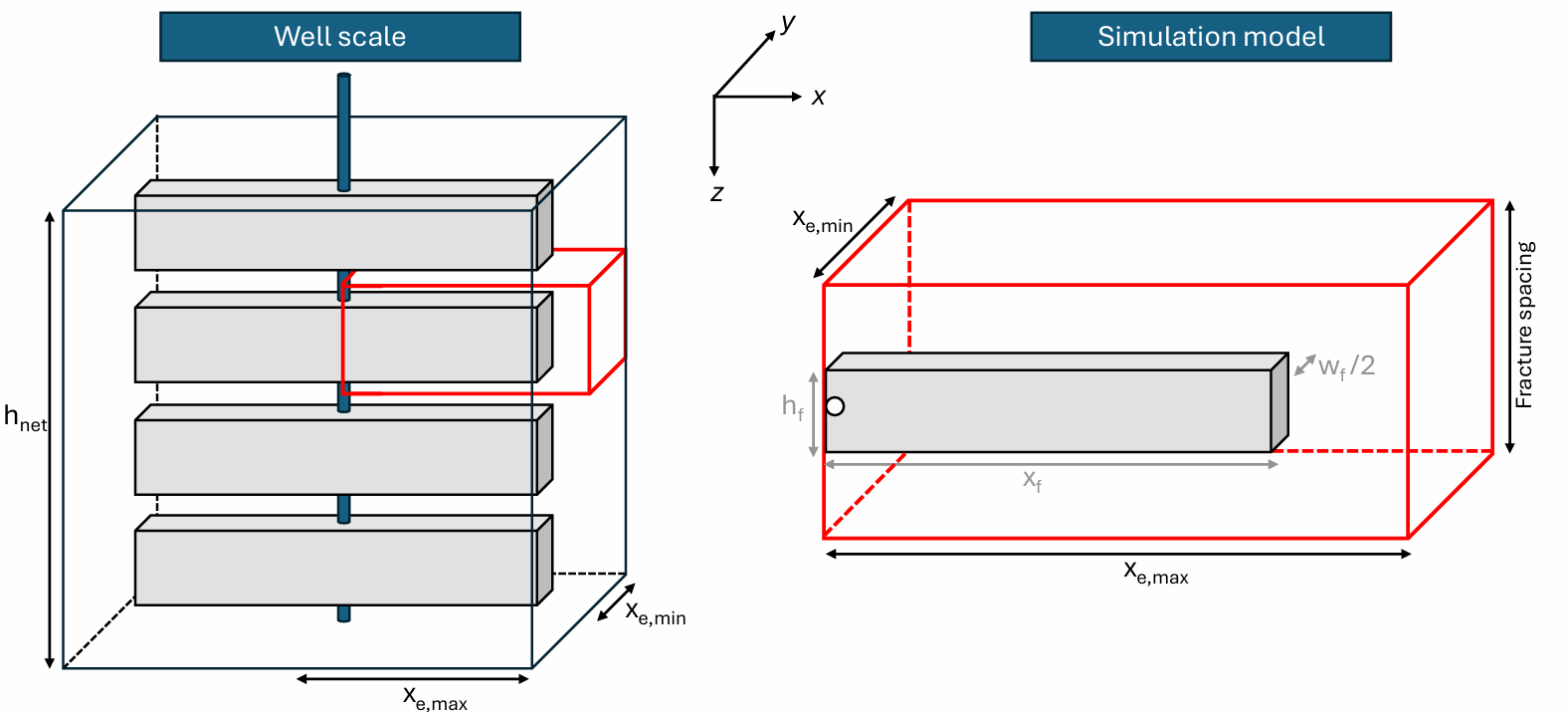
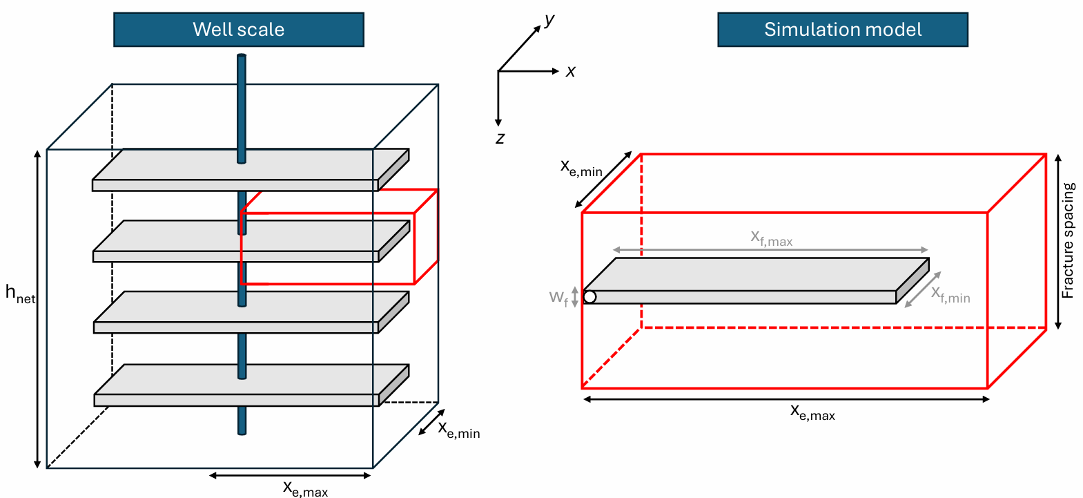
The simulations are performed on a prebuilt model that represents the typical well in tight unconventionals, often referred to as a multi-fractured horizontal well (MFHW). The prebuilt model is called the wellbox model. A cartoon of the wellbox model is shown below.
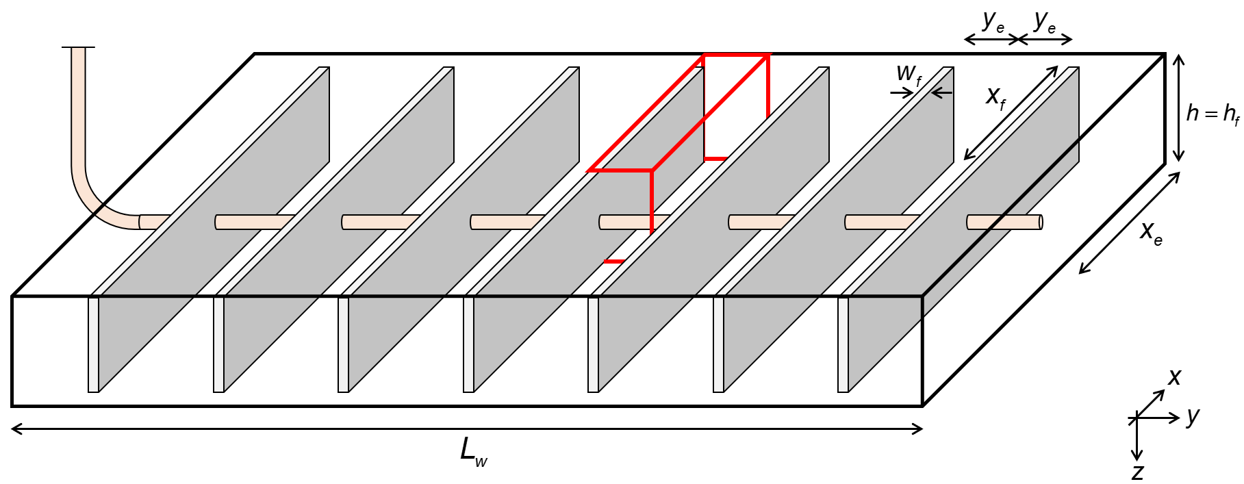
The wellbox model will have dimensions that the user can change, but a set of default values will be given initially. The dimensions and default values are as follows:
| Dimension | Symbol | Default Value |
|---|---|---|
| Lateral Length | 5280 ft | |
| Reservoir Half-Extent | 800 ft | |
| No. of Fractures | 100 | |
| Fracture Half-Length | 400 ft | |
| Reservoir and Fracture Height | 150 ft |
Note: The default wellbore diameter is 1 ft (corresponding to a wellbore radius of 0.5 ft).
As the wellbox model is symmetric, the numerical model will be a one-quarter fracture, as highlighted by a red-lined box in the figure above. The production from the numerical model is upscaled to by using a scaling factor. The scaling factor is defined as
where \(N_f\) is the number of hydraulic fractures (clusters) in the wellbox model. The dimensions of the numerical model are the same as the wellbox model, except for the y-dimension, where instead of \(L_w\), we use \(y_e\) defined as
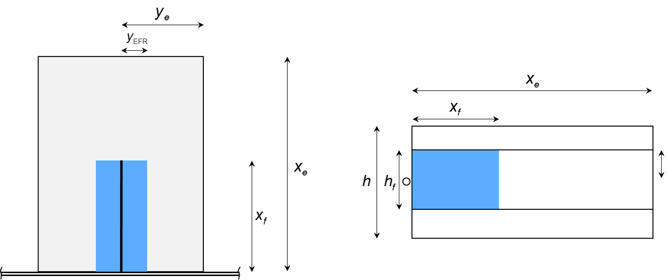
1.2. Enhanced Fracture Region (EFR) Option
It is possible to introduce a region of enhanced, effective permeability, \(k_{EFR}\), around each fracture with extent, \(y_{EFR}\). An example description for a single-fracture is illustrated in the figure below. The reservoir can extend beyond the fracture tip, and have contributions beyond the fracture height. The enhanced fracture region has the same height and length as the fracture, only difference being the extent in the y direction.
Pressure Dependent Permeability in the EFR region - Matrix gamma is applied to the EFR region, read more about pressure dependent permeability here.
1.2.1. EFR in whitson+
You can activate EFR in the model by toggling the EFR switch on in the 'Well and Reservoir Data' card. You will need to specify the extent of this EFR as a distance into the matrix from each fracture (less than the fracture spacing) for the enhanced permeability to be applied in this zone, as shown in the GIF below, where we add a 3ft EFR around the fracture with 10x matrix permeability:
When the EFR option is activated in whitson+, the LFP (A√k) reported in the Well & Reservoir Data card uses the EFR permeability (kEFR) instead of the matrix permeability (km) to calculate.
1.3. Reservoir Properties
1.3.1. Grid-Block Properties
The reservoir properties will include some properties that can be changed by the user, and some properties that are locked. The changeable reservoir properties are given the following table:
| Property | Symbol | Default Value |
|---|---|---|
| Matrix Porosity | 0.03 | |
| Matrix Permeability | 100 nd | |
| Matrix Initial HC Saturation (Fluid Dep.) | 1 | |
| Matrix Initial Water Saturation | ||
| Initial Reservoir Pressure | 7500 psia | |
| Hydraulic-Fracture Dimensionless Conductivity | 100 |
The locked reservoir properties are as follows
| Property | Symbol | Default Value |
|---|---|---|
| Fracture Porosity | 0.1 | |
| Fracture Width | 0.1 ft | |
| Depth | 10000 ft |
Note that depth is merely a cosmetic property as there is only one horizontal layer in the model, and no tubing calculations are made.
The dimensionless fracture conductivity is defined as
We calculate \(k_f\) from equation (3).
1.3.2. Saturation-Dependent Properties
1.3.2.1. Two-Phase Relative Permeability
The saturation-dependent properties in this model are the relative-permeability curves. We use the Corey-type model to express two-phase relative permeability. Baker's linear interpolation model is used to calculate \(k_{ro} = f(S_w,S_g)\) in three-phase systems.
The Corey-type model calculates \(k_{rw} = f(S_w), k_{row} = f(S_w)\), \(k_{rog} = f(S_g)\), and \(k_{rg} = f(S_g)\) as follows:
where the following parameters must be provided
| Property | Symbol | Default Value (Matrix) | Default Value (Fracture) |
|---|---|---|---|
| Connate Water Saturation | 0.2 | 0 | |
| Residual Oil Saturation (O-W) | 0.2 | 0 | |
| Residual Oil Saturation (O-G) | 0.2 | 0 | |
| Critical Gas Saturation | 0.05 | 0 | |
| Water Corey Exponent | 2 | 1 | |
| Oil Corey Exponent (O-W) | 2 | 1 | |
| Oil Corey Exponent (O-G) | 2 | 1 | |
| Gas Corey Exponent | 2 | 1 | |
| Water Relative Permeability at | 1 | 1 | |
| Oil Relative Permeability at | 1 | 1 | |
| Gas Relative Permeability at | 1 | 1 |
The relative-permeability values in the matrix will be open for change by the user. The fracture values are locked.
1.3.2.2. Three-Phase Relative Permeability
To achieve platform consistency between the different simulators (OPM Flow, Eclipse 100, Sensor, CMG IMEX), we have found that the Baker linear interpolation of \(k_{ro}\) is the only three-phase relative permeability that is common for all simulators.
The Baker linear interpolation correlation is as follows
The testing of OPM Flow has been done by comparing OPM Flow to Sensor. The default three-phase relative permeability correlation in Sensor is Stone 1 with Fayers' and Matthews' expression for \(S_{om}\). This option is not available in OPM Flow, which results in inconsistencies in predicted results for the two simulators. The default relative permeability correlation for OPM Flow (and E100) is the Baker linear interpolation. This correlation can also be activated in Sensor, making the two simulators consistent. However, Stone 1 with Fayer's and Matthew's expression for \(S_{om}\) remains the preferred choice, which was also the case for Keith Coats (see quote below)
The default three-phase relative-permeability correlation for CMG IMEX is Stone 2. Hence, for consistency, our output files to CMG IMEX format will contain a keyword activating the Baker linear interpolation correlation.
The table below summarizes the three-phase correlations available in the different simulators.
| Three-Phase Rel. Perm. Correlation | Sensor | OPM Flow | Eclipse 100 | CMG IMEX |
|---|---|---|---|---|
| Stone 1 | X | X | X | |
| Stone 1 with Fayer's and Matthew's | X | X | X | |
| Stone 2 | X | X | X | X |
| Baker | X | X | X | X |
Quote
"I would never use Baker kr. Stone 2 kr is pathological and Baker kr may be. To my knowledge Stone 1 – Fayers kr (sensor default) is the only kr logic free of pathology"
"Default kro is Stone 1 with Fayer’s modification. The ID option STONE 2 can be pathological, depending upon entered water-oil and gas-oil krow and krog relperm data. The pathology is a step-function change from kro>0 to kro=0 for an epsilon change in saturations. The default Stone 1 is not pathological"
*Default refers to Sensor
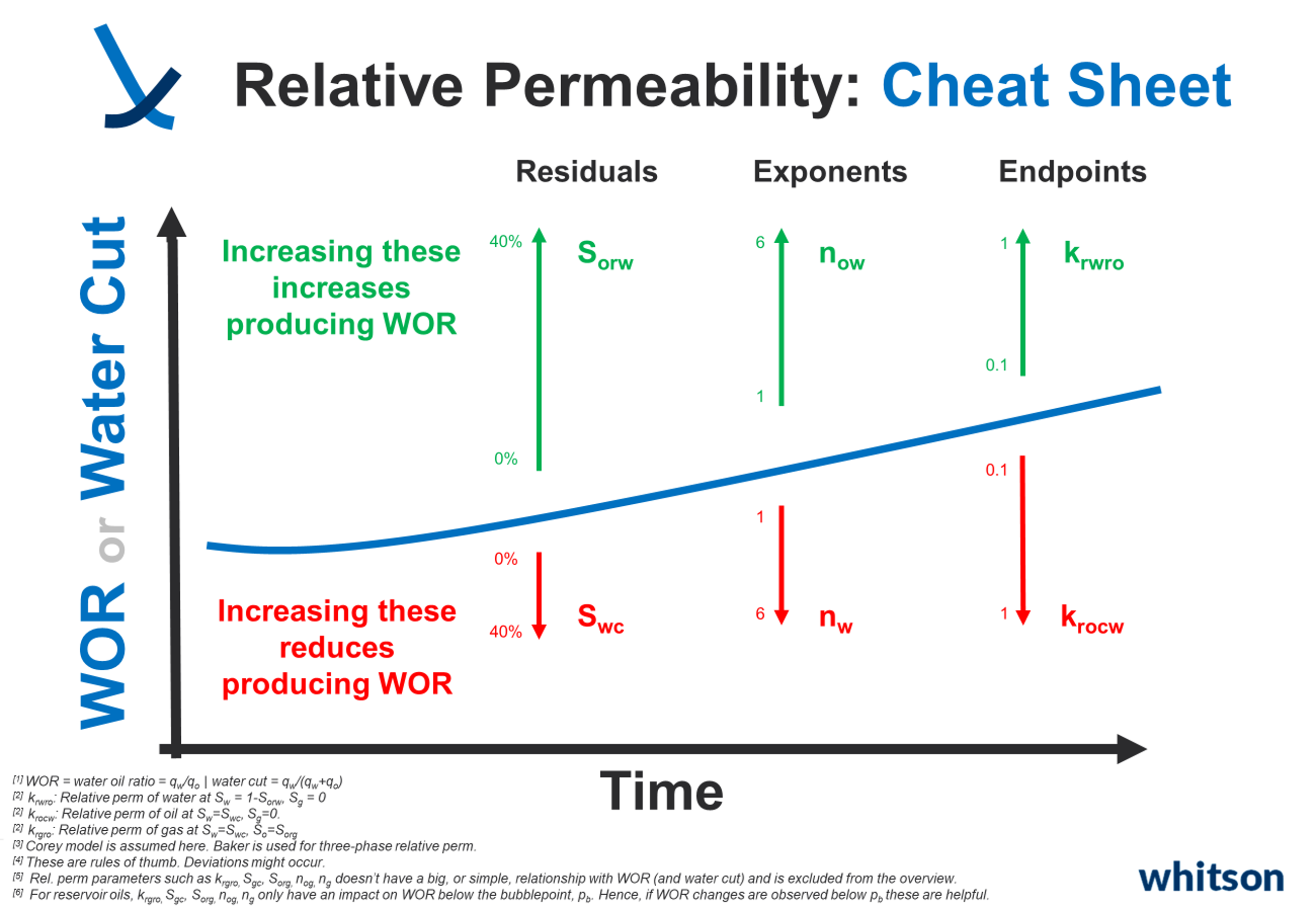
1.3.2.3. Relative Permeability and Producing Ratios
Understanding how relative permeabilities affect Gas-Oil Ratio (GOR) and Water-Oil Ratio (WOR), or water cut, can be tricky. It often takes experience, with engineers having their preferred parameters to tweak for achieving specific changes in simulated GOR, WOR, or other ratios. To simplify this, especially for beginners, we've created cheat sheets to help out.
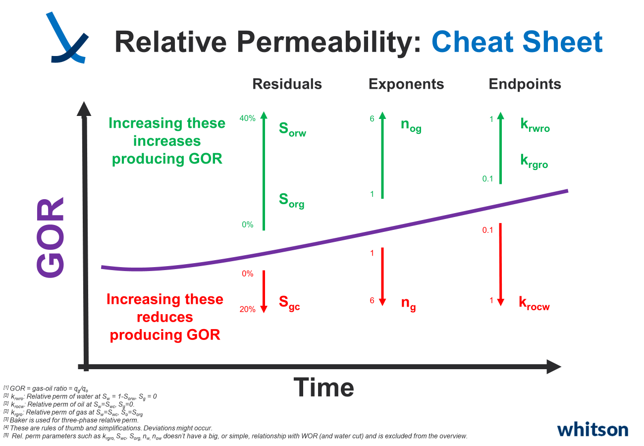
GOR and \(S_{org}\)
To understand the relationship between GOR and \(S_{org}\), it is necessary to take a look at the equation for producing GOR:
Just to simplify things slightly, it can assume that \(r_s\) is 0
The producing GOR is a combination of PVT properties and relative mobilities (\(k_{rg}\)/\(k_{ro}\)).
Reducing the \(S_{org}\), will reduce \(k_{rg}\)/\(k_{ro}\) (example below), and hence reduce producing GOR.
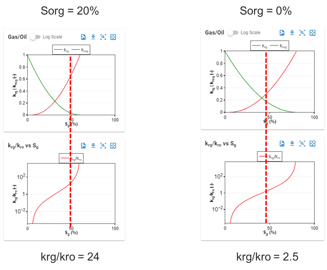
However, the relative reduction in \(k_{rg}\)/\(k_{ro}\) (and hence relative GOR reduction) will be a function of what the \(S_g\) is.
\(S_g\) is a function of fluid type (i.e. less gas comes out of solution of a low GOR oil with \(R_{si}\) = 500 scf/STB vs a near-critical fluid with \(R_{si}\) = 3500 scf/STB).
For the example below:
- If e.g. \(S_g\) is 50% (i.e. a more gassy fluid), the difference by changing \(S_{org}\) down to 0% would mean a reduction in \(k_{rg}\)/\(k_{ro}\) from 24 down to 2.5 (example). Order of magnitude difference.
- If e.g. \(S_g\) is 10% (i.e. a less gassy fluid), the difference by changing \(S_{org}\) down to 0% would mean a reduction in \(k_{rg}\)/\(k_{ro}\) from 0.01xx to 0.01yy (example). Almost no difference.
1.3.2.4. Relative Permeability in whitson+
Here's how you can adjust the relative permeability for your numerical model and visualize the rel-perm curves set up from these settings. Be sure to run the numerical model after editing the relative permeability table for the updated curves to be databased and displayed.
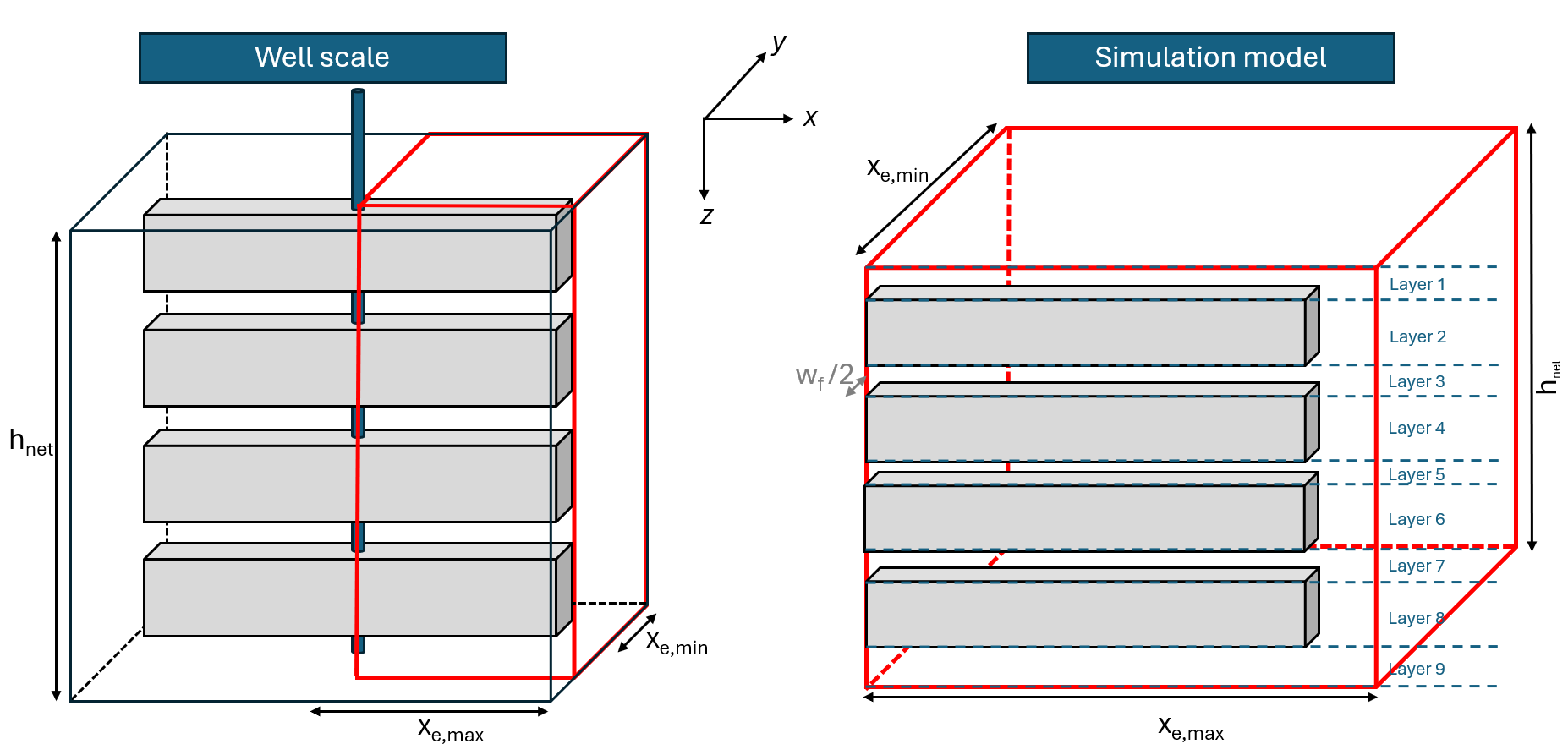
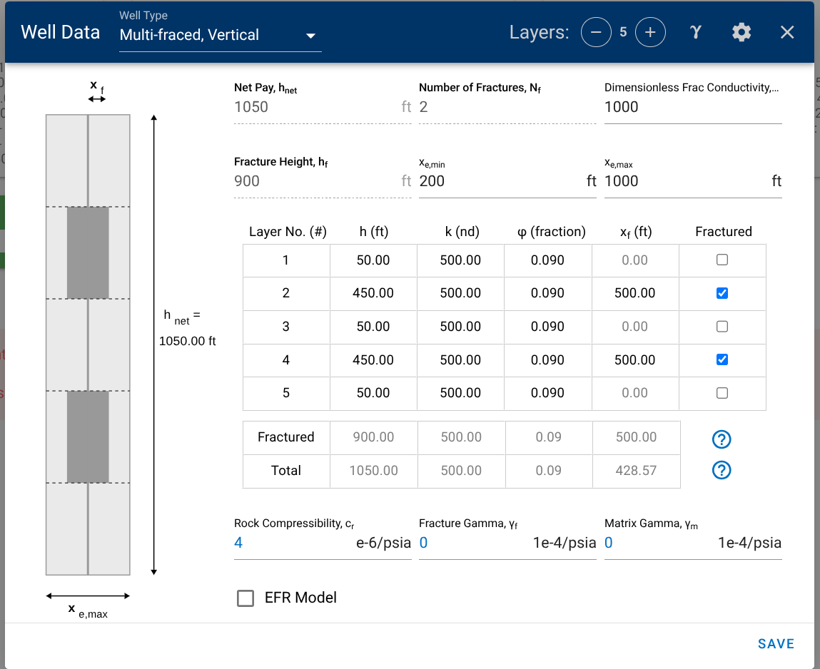
1.3.3. Multi-Layer Models
In whitson+, it is possible to have more than a single layer in the model with fully or partially penetrating fracture.
The fractured layer properties are calculated by height weighted average of the \(n\) penetrated layers, as follows
1.3.3.1. Multi-layer model, multi-fluid initialization in whitson+
You can not only set up a multi-layer model as outlined above, but you can also initialize PVT for each layer independently. You can set up each layer with its own fluid composition and black oil tables, that will be used to simulate phase mobility in each layer separately. Typical uses may include modeling water breakthrough as layers with 100% water saturation, etc. The steps to create multi-layer, multi-fluid models are outlined in the GIF below, where we add 2 additional layers and set up PVT such that there is only gas contribution from the layer on top and water contribution from the bottom layer:
1.4. Fluid Properties
whitsonʳˢ is designed to do simple and fast reservoir modeling to evaluate depletion performance. To make this tool as efficient as possible, the modified black-oil PVT model (outlined below) is used for the fluid treatment. An important feature of whitsonʳˢ is the direct link to whitsonᴾⱽᵀ. This makes the generation of black-oil PVT tables a backend feature in whitsonʳˢ, where the user only needs to provide key properties related to fluid PVT such as temperature, surface-process information (separator pressure and temperature), and initial gas/oil ratio.
The key parameters of the modified black-oil PVT model are (details and definitions are found in Whitson and Brulé 2000) as follows:
| Property | Symbol |
|---|---|
| Oil Formation Volume Factor | |
| Solution Gas/Oil Ratio | |
| Dry-Gas Formation Volume Factor | |
| Solution Oil/Gas Ratio | |
| Oil Viscosity | |
| Gas Viscosity |
whitsonʳˢ will return the in-place volumes of the wellbox model when all model dimensions, reservoir properties, and fluid properties have been specified. The in-place numbers are calculated as
1.4.1. Effect of on Inplace Calculation
The numerical model represents a one-quarter-fracture symmetry element. The simulated rates from this symmetry element are then upscaled to obtain the full-well production profile. The lateral extent of the matrix portion of each symmetry element is defined as:
In principle, the total fluid in place for the full-well model is controlled by the reservoir dimensions and should not be directly dependent on the number of hydraulic fractures. However, the numerical model explicitly represents each hydraulic fracture as a gridded fracture element connected to the adjacent matrix grid block. As a result, changing Nf changes the number of fracture grid elements included in the full-well upscaled model. Because each gridded fracture element has an associated pore volume, this may introduce a very small change in the calculated fluid in place when the number of fractures is modified. This effect is typically negligible because the fracture pore volume is small compared with the matrix pore volume.
1.4.2. How to Handle Simulation of Different pRi and GORi?
The black-oil PVT table is always generated in whitsonʳˢ from initial composition (), reservoir temperature (), equation of state (EOS), and surface process configuration. The black-oil PVT table is always regenerated locally at runtime, taking only a fraction of a second. This approach ensures flexibility and avoids delays previously encountered when downloading pre-generated BOT files from the cloud.
Current handling for variations in initial reservoir pressure () and initial GOR ():
The black-oil PVT table is primarily a function of (through ) and (). The is used to initialize the fluid as either single-phase or two-phase. This parameter is not a direct input in the generation of the black-oil PVT table but is used during its extrapolation to avoid numerical instabilities of negative compressibility and internal extrapolation as much as possible. Therefore, the extrapolated part of the black-oil PVT table (affected by ) is typically outside the region used in simulations and should not materially impact the quality of the results.
-
Variations in with fixed
When is held constant, the same is used across all cases. Varying influences the initialization of the fluid system:
-
If ≥ , the fluid initializes as single-phase.
-
If ≤ , the fluid initializes as two-phase.
Effects of Varying with Fixed
If you compare the files of two History Matching cases with same , but different , there may also be some differences in the extrapolated part of the black-oil PVT table, but that should not impact the simulations.
-
Variations in with fixed
Changing is equivalent to altering the . For each case, black-oil PVT table will be generated using different composition. A new composition () is generated by taking the original obtained from Fluid Definition and recombining it to match the specified . A new BOT is then constructed based on () and used in the simulation.
-
Variations in both and
Both effects described in previous points are applied simultaneously.
1.5. Water and Rock Properties
The following water and rock properties are used as default values for all reservoir simulators.
| Property | Symbol | Default Value |
|---|---|---|
| Water Formation Volume Factor at & | 1 RB/STB | |
| Water compressibility | 3×10 1/psia | |
| Surface water density | 62.37 lb/ft | |
| Water viscosity | 0.5 cp | |
| Reference pressure for | 14.696 psia | |
| Formation (rock) compressibility | 4×10 1/psia |
1.6. Geomechanical Effects - Pressure-Dependent Permeability
The matrix, EFR (if activated), and hydraulic fracture can be assigned a pressure-dependent permeability on the form where \(\gamma\) is a property that be assigned in the frontend. There are two different gamma values, on for the hydraulic fracture \(\gamma_f\), and one for the matrix and EFR (if activated) \(\gamma_r\). To activate the pressure-dependent permeability, toggle on "Pressure-Dependent Permeability" under the "Well & Reservoir Data" card in the "History Matching" module.
For a given dataset, a higher gamma value—reflecting productivity loss due to pressure-dependent permeability—requires more / to achieve the same and production rate.
1.6.1. Pressure-Dependent Permeability in whitson+
Pressure dependent permeability can be added as a gamma value to the matrix and EFR(\(\gamma_r\)), and the fracture(\(\gamma_f\)) by bulk editing multiple wells (Well Overview page), directly in the well headers (Scenarios page), or by using input fields in NRTA and Numerical Model features - your changes to \(\gamma\) in any one of these places should be reflected in all other places.
You can visually set it up in the numerical model by specifying only the gamma to be used in the exponential relationship above to calculate and display the plot of permeability as a function of pressure. If you have tabulated data for the formation permeability at different pressures, you can also use the table directly to set up an interpolation for the permeability as a function of pressure.
You can include pressure dependent permeability as outlined in the GIF below:
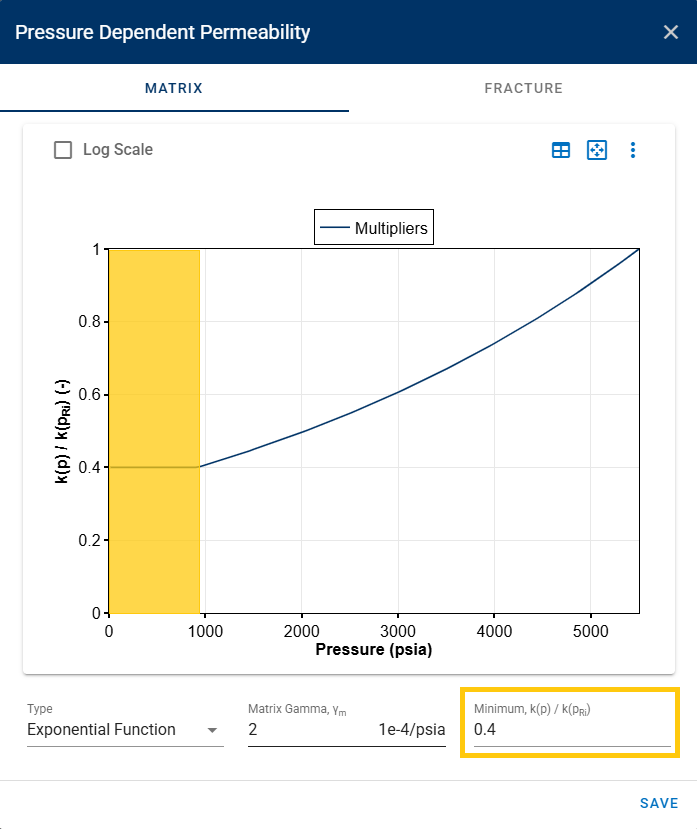
1.6.2. Minimum Permeability Multiplier
To model more realistic pressure-dependent permeability behavior, the simulation includes a setting for a minimum permeability multiplier, \(k(p)/k(p_{ri})\). This defines the lowest allowable permeability relative to the reference pressure.
For example, by specifying a value of 0.4, the permeability is prevented from dropping below 40% of its original value, even at low pressures. This helps capture the fact that in many formations, permeability loss stabilizes at lower pressures due to rock compaction limits, rather than continuing to decline indefinitely.
1.7. Computing Original Gas in Place with Adsorption
Shale reservoirs possess a remarkable capacity to store methane through a process known as "adsorption." This involves gas molecules adhering to the organic material within the shale, creating a near-liquid state of condensed gas. A useful analogy is to envision a magnet sticking to a metal surface or lint clinging to a sweater, illustrating the concept of adsorption versus absorption, where one substance is trapped inside another like a sponge soaking up water. The adsorption process is reversible due to its reliance on weak attraction forces.
Compared to conventional reservoirs, shale reservoirs can store significantly more gas in the adsorbed state, even when compression is applied at pressures below 1000 psia. Notably, the gas stored in shale is predominantly held in the adsorbed state, as opposed to being free gas. This is because the volume of the cleat or fracture system within shale is relatively small compared to the overall reservoir volume. As a result, the pressure volume relationship is commonly described through the desorption isotherm alone.
Langmuir Isotherm
The release of adsorbed gas is commonly described by a pressure relationship called the Langmuir isotherm. The Langmuir adsorption isotherm assumes that the gas attaches to the surface of the shale, and covers the surface as a single layer of gas (a monolayer). At low pressures, this dense state allows greater volumes to be stored by sorption than is possible by compression.
The typical formulation of the Langmuir isotherm is:
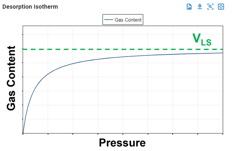
Langmuir Volume, VLS
The Langmuir volume is the maximum amount of gas that can be adsorbed by a shale at an "infinite pressure". The plot below of a Langmuir isotherm demonstrates that gas content asymptotically approaches the Langmuir volume as pressure increases to infinity.
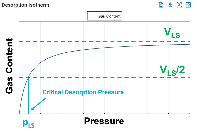
Langmuir Pressure, pLS
The Langmuir pressure, or critical desorption pressure, is the pressure at which one half of the Langmuir volume can be adsorbed. As seen in the figure below, it changes the curvature of the line and thus affects the shape of the isotherm.
Computing Original Gas in Place (OGIP)
Ambrose et al.[1] argue that the free OGIP must be corrected for the adsorbed gas that occupies some of the hydrocarbon pore volume (HCPV). If porosity is estimated from core plugs where core preparation has removed the adsorbed gas, then the OGIP will be overestimated.
The convention of reporting OGIP when adsorption is included, is to report it in units of scf/ton (standard cubic feet per short ton). For a fluid system having only dry/wet gas and water, the total OGIP is
where
and with \(C_1\approx 5.7060\) and \(C_2\approx1.318\cdot10^{-6}\) are unit conversion factors. The shale saturation is capped at \(1-S_{wi}\), meaning the maximum amount of shale you can have is the entire HCPV. Hence, this will make the results independent of the adsorption numbers when violating this constraint.
The OGIP resolved in the ARTA and GFMB features yields the free OGIP. We can use this volume to compute the rock mass, which in turn can be used to calculate the adsorbed OGIP. Multiplying equation \eqref{eq:freegasperton} with the rock mass (\(G=\hat{G}_f m_r\)) gives the free OGIP in units of scf. Solving for the rock mass yields
This rock mass can then be multiplied by equation \eqref{eq:adsorbedgasperton} to get the adsorbed OGIP in scf, i.e.,
Total Compressibility when Adsorption is ON
In order to honor mass balance, it becomes necessary to modify total system compressibility when accounting for adsorption. Total system compressibility can be determined using the following equation:
The derivation of this equation is shown here and is constructed upon Ambrose et al.[1].
Adsorption in whitson+
By default, the adsorption feature is turned off for all the wells and is only available for use in gas wells. Here's how to activate the adsorption feature in whitson+ and set up the langmuir isotherm for your gas well:
2. Numerical Model
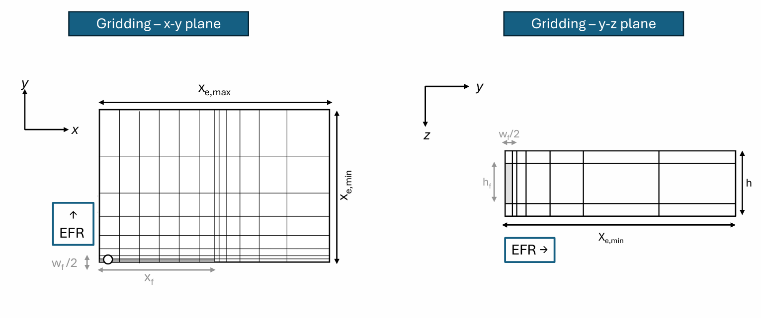
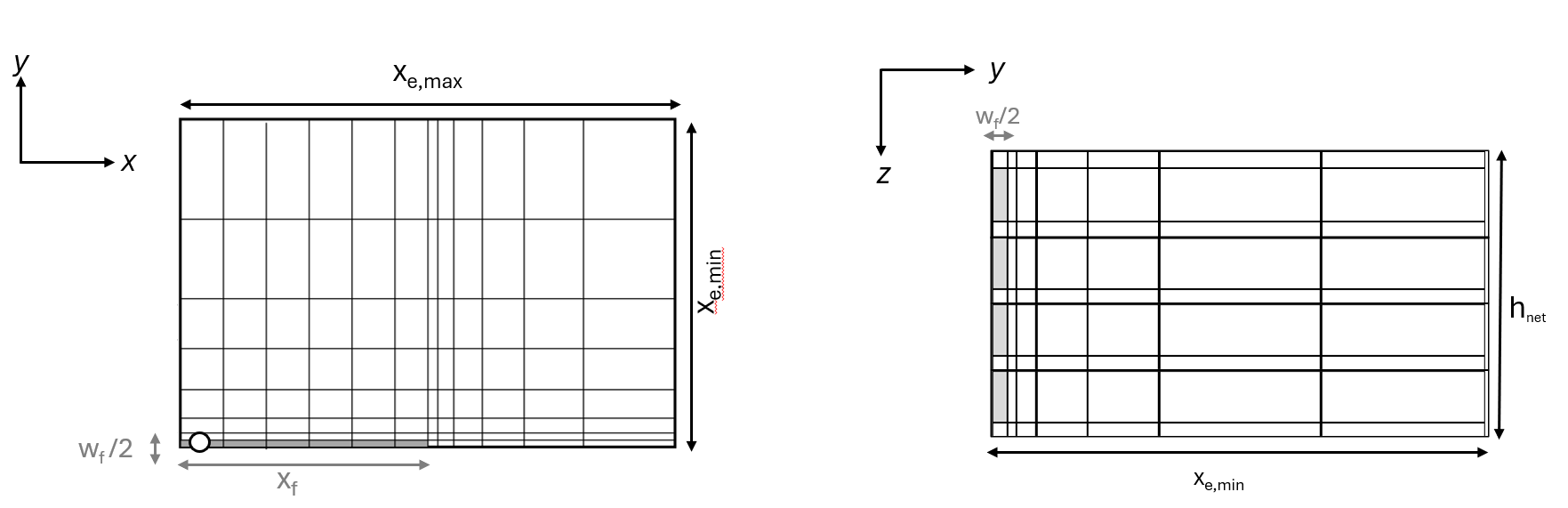
2.1. Gridding
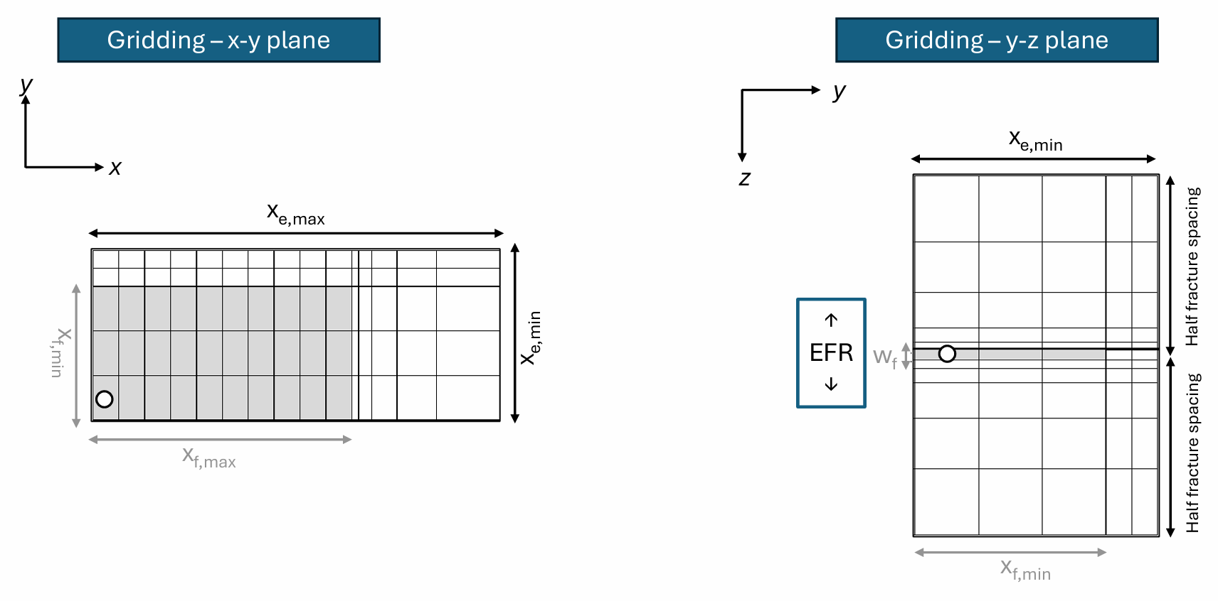
The numerical model will have a gridding as shown in the figure below. The gridding is logarithmic in the y-direction, and in the x-direction beyond the fracture tip. From the wellbore to the fracture tip the gridding is uniform in the x-direction.

The gridding is calculated based on the dimensions of the model. The gridding of the numerical model is a backend feature, where the user can choose between low, medium, and high grid refinement. Determining the number of grid blocks for the chosen level of grid refinement is discussed in the next subsection. The formulas used for gridding are
where the total number of grid blocks in the model are \(N_t = (N_{x,i} + N_{x,o})N_y = N_xN_y\).
Changes to the default grid
The gridding described above is for the default symmetry-element MFHW model.
- Adding an EFR region to the model will change the grid to Cartesian in the y-direction from the fracture to the EFR boundary, and logarithmic beyond. This change to the grid can cause different results when \(k_{EFR} \rightarrow k_m\). This is merely an artifact of the gridding, and increasing the grid-refinement level will minimize the difference.
2.2. Grid Refinement
The number of grid blocks in the model is controlled by the grid-refinement level set by the user. There are four levels of grid refinement which allow the user to decide the level of "compromise" between simulation run time and level of detail captured in the simulation results:
- Very Low (favours short simulation time)
- Low
- Medium
- High (favours capturing the details)
An internal logic is used to translate the level of grid refinement to a number of grid blocks. We use average grid-block dimensions in the \(x\)- and \(y\)- directions to set the refinement of the gridding. The following table contains the fixed numbers for \(\bar{\Delta} x\) and \(\bar{\Delta} y\) at the three grid-refinement levels.
| Property | (ft) | (ft) |
|---|---|---|
| Very Low | 200 | 8 |
| Low | 50 | 2 |
| Medium | 25 | 1 |
| High | 12.5 | 0.5 |
The number of grid blocks in the \(x\)- and \(y\)- directions are then calculated as
The split of grid blocks in the \(x\)-direction \(N_{x,i}/N_x\) is linear with \(x_f/x_e\). Because the number of grid blocks have to be integers, we round the numbers as follows:
The number of grid blocks outside the fracture tip are then calculated by \(N_{x,o} = N_x - N_{x,i}\).
2.3. Grid Outputs - Pressure, Saturation 2D Maps
Grid refinement used in the previous section dictates the number of grid blocks used in the simulation model. Each gridblock can have the following results as outputs from the full-physics numerical simulation - pressure, oil, gas and water saturations - at discrete timesteps, spanning the simulated production history and forecast. Such maps with pressure and phase saturations for each gridblock can be used to estimate the drawdown and depletion across different parts of the model.
2.3.1. Choosing Grid Refinement and Using 2D Maps in whitson+
You can set whether you want to capture this information prior to running the simulation by toggling on the 2D Map button on the top-right of the screen - this will prompt you to rerun the simulation so that the results can be captured. Once the model is rerun, clicking the 2D Map button will open the pressure and saturation maps collected during the run.
You can visualize the results with 10 fractures together or look at a single fracture model in two ways:
- In bird's eye view, i.e. the x-y cross-section or each layer along the z direction in multi-layer models, and
- In side view, i.e. the z-y cross-section or layers along the x direction (i.e. fracture half-length, wellbore to fracture tip).
You can even set up fixed ranges for the colorbar manually, so that the colorbar limits do not change dynamically for each timestep.
Be sure to rerun the numerical model every time you change the grid refinement since this sets up a new discretization of the model and the grid output maps will be different due to the difference in the number of grid blocks. Here's how to activate 2D maps - notice how using a higher grid refinement offers higher resolution maps with more grid blocks, compared to low or very low grid refinements in the GIF below:
2.4. Well Control
A well is always controlled by specifying a target rate. The most common rate is a surface product rate such as surface gas rate, surface oil rate, or surface water rate. Sometimes the target is a phase rate specified at flowing bottomhole conditions, either as a single-phase wellbore rate, or a combination of several wellbore phase rates, e.g. "reservoir" wellbore oil phase rate, "reservoir" wellbore liquid (oil phase + water phase ) phase rate or total wellbore fluid rate (gas phase + oil phase + water phase).
A zero target rate can also be specified, meaning that no production is seen at the surface. The well is "shut-in" at the surface. Downhole within the wellbore, considerable flow rates usually are found during the shut-in of a well with multiple well connections (to >1 grid cells). Some well connections show positive production rates and other well connections experience negative injection rates. The total injection rate of all components (surface gas, surface oil, surface water) must equal the sum of all well connection production product rates (to ensure no material balance loss in the wellbore during a shut-in time step).
The well tries to satisfy the target rate during a time step, but only if the specified pressure constraint is not violated. Typical pressure constraints include flowing bottomhole pressure or flowing tubing pressure. If the pressure constraint is reached then the target rate can not be met and a rate is chosen that ensures the pressure constraint exists in the well.
During zero target rate and STOP (i.e. well closed at the surface), the pressure constraint will be honored. Layer crossflow may happen if the well is connected to multiple numerical layers with differential depletions. During zero target rate and SHUT (i.e. well closed at the sand face), the well is isolated, no well constraint is enforced.
A producing well can also have constraints on the well's produced surface product ratios GOR, WOR, OGR, surface water cut of total liquid rate or reservoir wellbore phase fractions such as water cut. These constraints are usually maximum values which, if reached, the wellbore pressure is adjusted to honor the constraint, and accordingly not allow the target rate to be met.
2.4.1. Well Control in whitson+
There are six options currently available for controlling wells:
| Constraint | Description |
|---|---|
| Oil | Maximum surface oil production rate target or constraint. |
| Gas | Maximum surface gas production rate target or constraint. |
| Water | Maximum surface water production rate target or constraint. |
| Liquid | Maximum surface liquid (oil + water) production rate target or constraint. |
| BHP | Minimum bottomhole pressure target or constraint. |
| BHP (synthetic) | Bottomhole pressure profile target or constraint, with an option to include a maximum rate constraint. The BHP profile is defined by user inputs such as: (a) minimum BHP, (b) time to minimum BHP, and (c) total simulation days. |
During the historical period, the well is controlled on the user-selected option. If the well is controlled by one of the surface-rate targets, then a BHP constraint of 100 psia is applied. If the well is controlled on a BHP target, then the software will set an unrealistic rate target with the desired BHP profile as a lower limit for producers. For the synthetic BHP profile, there has, since the Sept. 2023 release of whitson+, been an option of setting a rate constraint.
During shut-ins period, the status of the well is set to STOP, indicating no fluid production to the surface and potential layer crossflow may occur if there are any open connections.
During the forecast period, the well is consistently controlled based on either a BHP or WHP (CHP or THP) target, with the added flexibility of applying a maximum rate constraint. If none of rate constraint is chosen, then the rate will be set to an unrealistic target.
It is important to note that whitson+ does not support "Reservoir" or bottomhole-rates targets. Additionally, constraining the well based on producing ratios (GOR, WOR, OGR, GLR, etc.) is also not supported. No economic criteria for production wells are currently being enforced. This implies that the well will only be shut-in (denoted by a well status of STOP) if the well has zero rates and/or the pressure falls below the predefined minimum bottomhole pressure (whitson+ default is 100 psia).
Should your company require any of these constraint options, please feel free to contact us or use the Send Feedback button at the top right of whitson+.
2.4.2. How does whitson+ recognize a shut-in?
| Well Control | Shut-in Condition |
|---|---|
| Oil | The well is shut-in if the oil rate for the time step is zero. |
| Gas | The well is shut-in if the gas rate for the time step is zero. |
| Water | The well is shut-in if the water rate for the time step is zero. |
| Liquid | The well is shut-in if the liquid rate (oil + water) for the time step is zero. |
| BHP | The well is shut-in if all production rates (oil + gas + water) for the time step are zero. |
Interpreting Zero Rate Profiles
Should all the rates for all time steps be uniformly zero, the software assumes that the user would like to control the model on a custom, uploaded BHP profile. Consequently, the well won't be considered as shut-in.
2.5. Time Stepping
The selected well control and grid refinement is used to run the simulation model and Time-Stepping dictates how many timesteps should be passed to the simulator.
Higher number of time-steps takes longer to run since the simulator tries to match the given well control for all these time steps. A significant reduction of the model run-times can be achieved with a negligible trade off in model accuracy - which is especially useful for wells with long, noisy producing history or BHP. Here are the available options to control the number of timesteps to use for simulation:
| Option | Description |
|---|---|
| All | Simulates every uploaded timestep without skipping any points. |
| Smart | Simulates daily timesteps for the first 100 days, then every 10th timestep afterward. |
| Custom | Simulates every Nth timestep, where N is user-defined. For example, setting N = 7 will simulate weekly timesteps. |
2.6. Fracture Conductivity as a Function of Distance and Fracture Angle
2.6.1. Fracture Conductivity as a Function of Distance - Fcd(x)
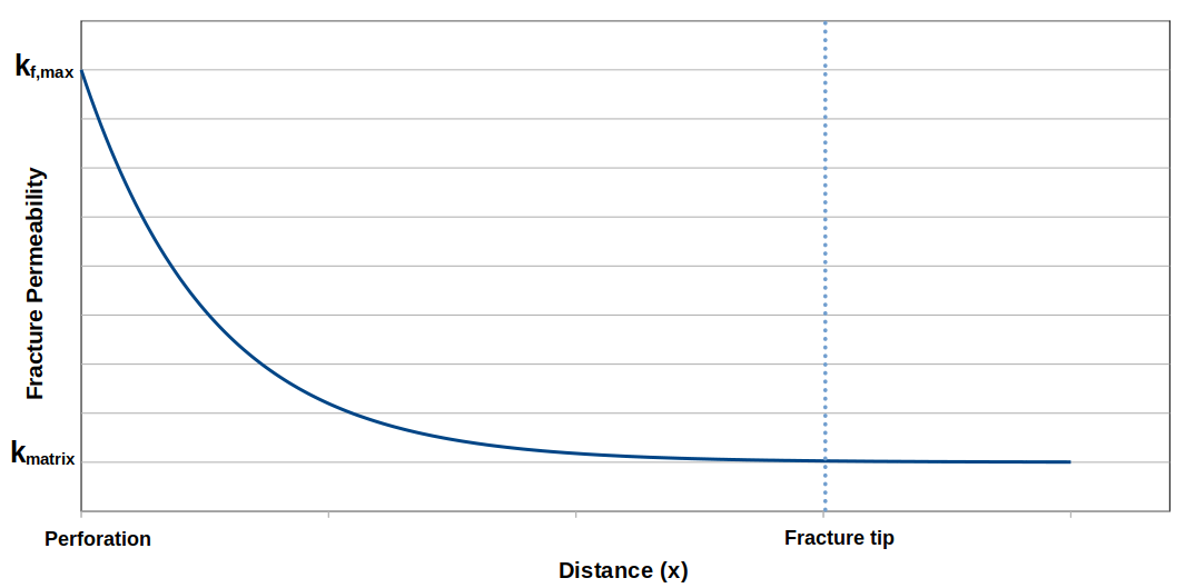
Fracture conductivity can be modeled as a function of distance, with the maximum fracture permeability occuring at the perforation point and gradully decreasing toward the fracture tip.
\(\kappa\) represents the conductivity decline factor in \(1/ft\). Fracture conductivity is used to calculate fracture permeability as outlined in Eq. \eqref{eq:dimlessfraccond}. By rearranging Eq. \eqref{eq:fcdx} with Eq \eqref{eq:dimlessfraccond}, fracture permeability can be calculated as follows
In whitson+, we use harmonic average to calculate the permeability across the grid cell to get the cell-average permeability.
where \(a\) is \(x_{min}\) and \(b\) is \(x_{max}\). Activating this option requires the user to input conductivity decline factor \(\kappa\)
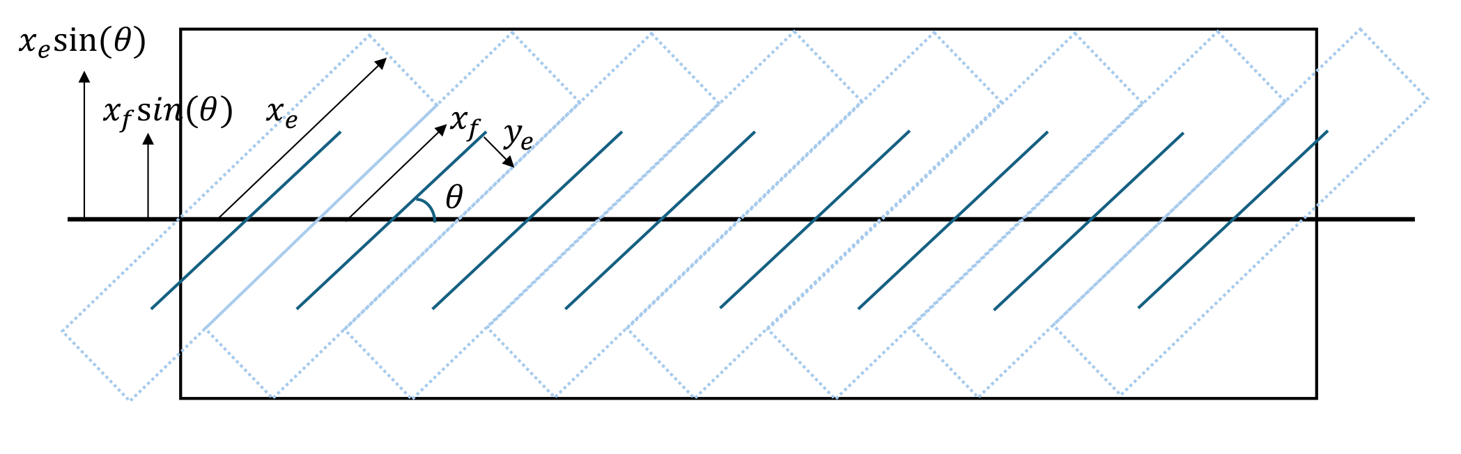
2.6.2. Fracture Angle
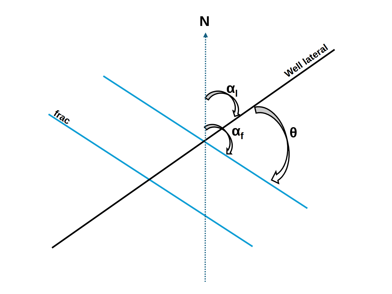
Activating this option requires the user to input well lateral \(\left(\alpha_l\right)\) and fracture azimuth \(\left(\alpha_f\right)\) relative to North. The difference between well lateral and fracture azimuth is referred to as the fracture angle relative to lateral \(\left(\theta \right)\). By default, the fracture is assumed to be perpendicular to the lateral \(\left(\theta = 90^{0}\right)\). This input determines how the fracture spacing is modeled in the simulation.
The figure below illustrates the adjustment of the symmetry element model in relation to \(\theta\).
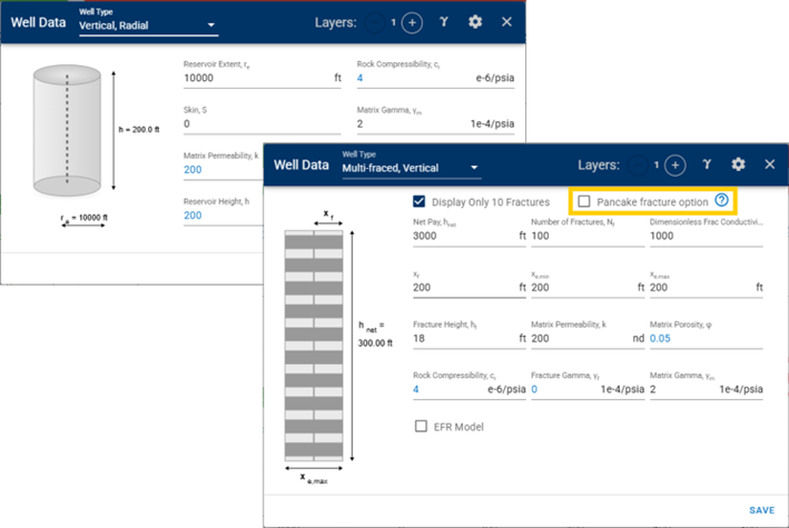
2.7. Numerical Well Models
The software provides multiple numerical well models to represent different well configurations and reservoir flow geometries in simulation, ranging from classical radial flow to explicit fracture-driven behavior. Available options include Vertical, Radial and Multi-Fractured, Vertical well models, with an optional Pancake Fracture representation.
2.8. Advanced Settings
2.8.1. Traditional PVT Formulation
This option enables to use PVDG (PVT properties of dry gas without vaporized oil) in the simulation instead of the default setting, PVTG (PVT properties of wet gas with vaporized oil). This option can be applied in scenarios where the CGR (Condensate-Gas Ratio, \(R_v\)|\(r_s\)) term is considered negligible, allowing it to be omitted from the PVT table. While this approach is not 100% accurate, it is often favored for its computational efficiency, especially with lower GOR oils. It will only work for fluids without nonmonotonic gas formation volume factor (\(B_g\)), a condition typically observed in near-critical fluids. That being said, this option is not recommended for gas condensate wells.
2.8.2. SWOF-SGOF Option
There are two distinct families of relative permeability models. The first family is SWOF and SGOF where the oil relative permeabilities are in the same tables as the water and gas relative permeabilities. The second family is SWFN and SGFN where this requires the oil relative permeabilities in a separate table (SOF3). By default, whitson+ utilizes the second family. This option allows the user to use the first family.
While there is typically no difference in results for oils, gas condensates or wet gases, minor variations might arise in specific cases. One keyword family may be preferred over the other when exporting results to simulation environments outside of whitson+.
3. What affects producing GOR profile and how?
3.1. Reservoir Parameters
We observe a wide-range of producing GOR profiles in tight unconventionals. But which reservoir parameters change producing GOR when the bottomhole pressure is below the saturation pressure? And how?
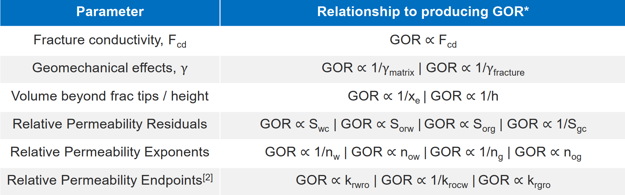
There are four broad categories of reservoir parameters that impact producing GOR
- Fracture conductivity
- Geomechanical effect
- Contributing volume beyond frac tips / height ("unstimulated rock")
- Relative permeability
This is summarized in the table above. Read more in this slide deck here.
3.2. Flow Regime
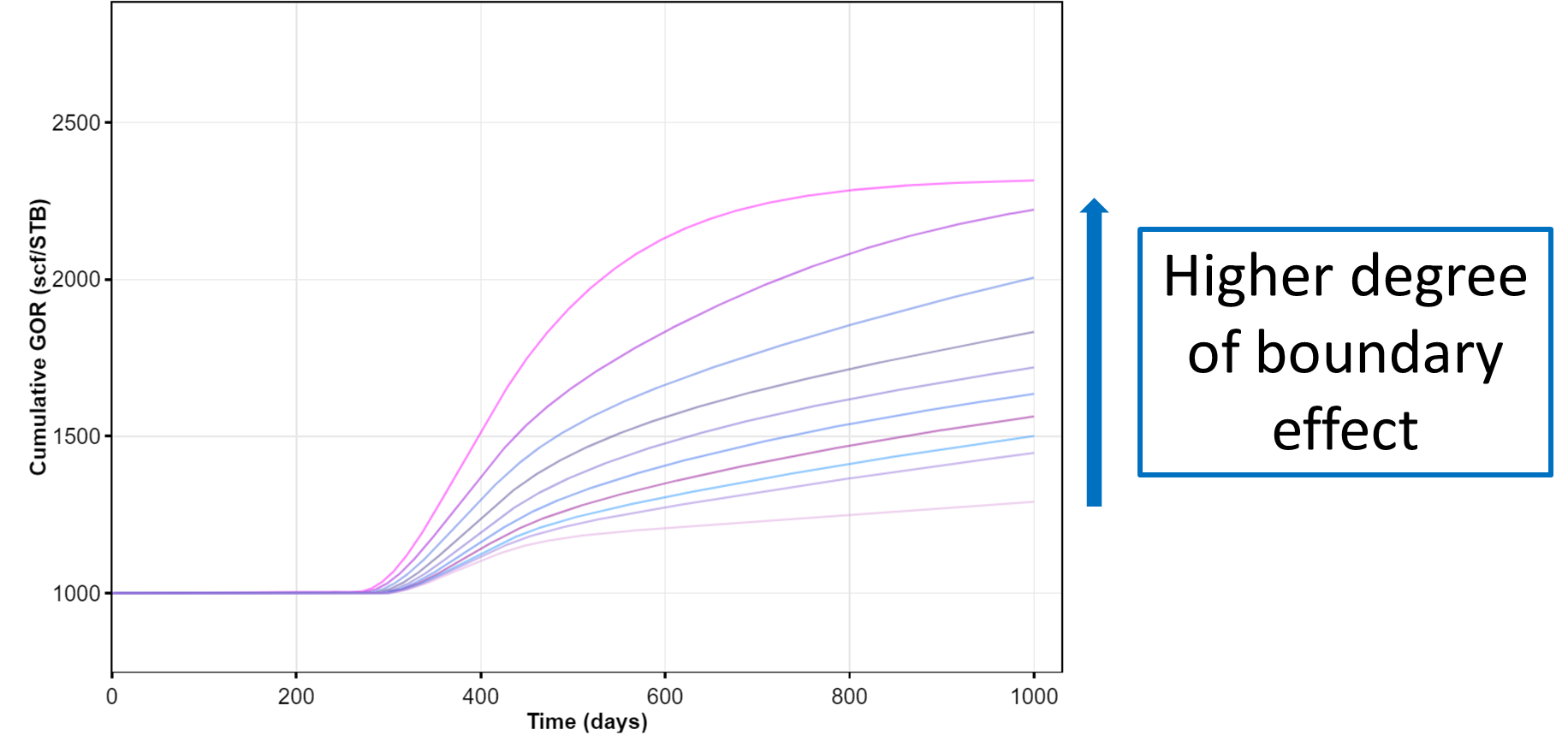
In addition to the reservoir parameters outlined above, flow regime matters. Everything else being equal producing GOR follows this relationship below saturation pressure:
Where IA refers to infinite acting, TF refers to transitional flow and BDF refers to boundary dominated flow.
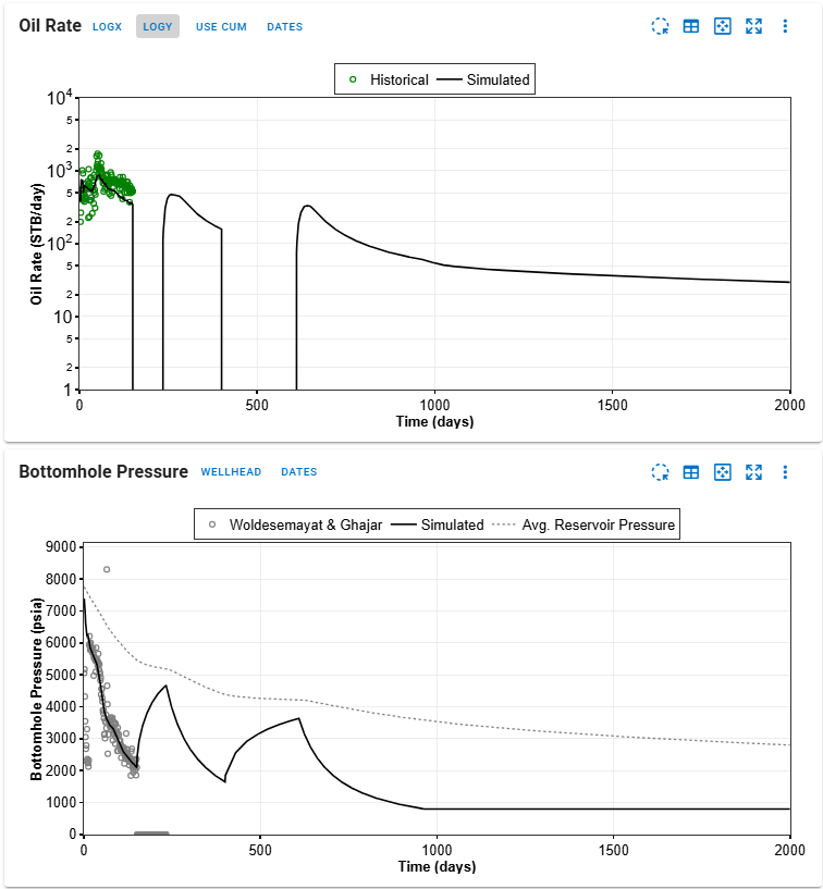
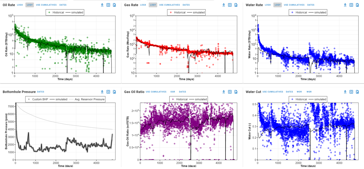
4. Why do rates spike at bubblepoint?
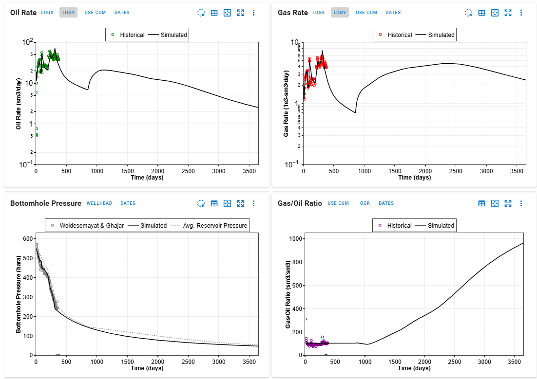
The rate spikes result from solution gas drive and a large LFP/OOIP ratio (larger permeabilities/lower contacted pore volumes). The \( p_{wf} \) and \( p_{avg} \) values are observed to be approaching a common value (see image above).
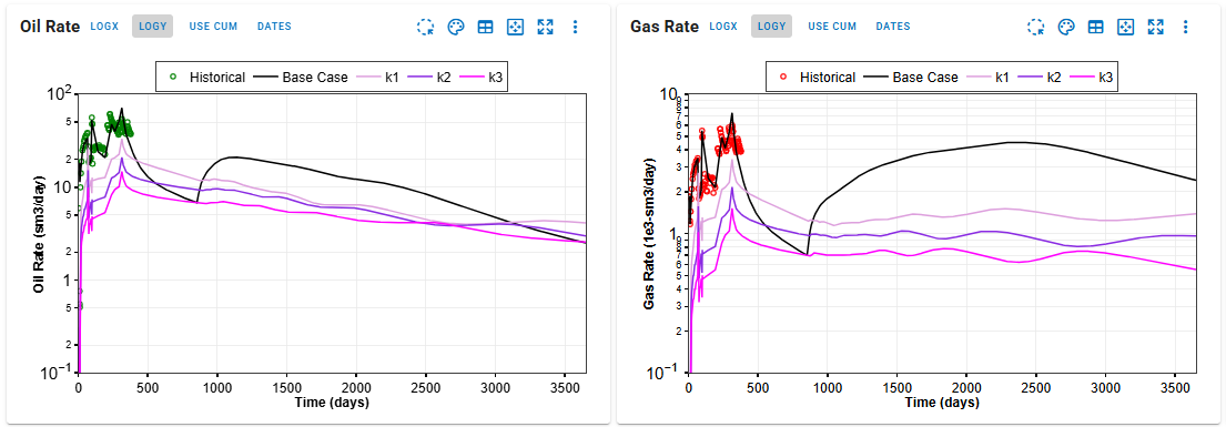
Mitigation of the rate kicks can be achieved by lowering the LFP/OOIP ratio, through either a reduction in permeability, an increase in pore volume, or a combination of both.
For example, maintaining a constant contacted pore volume while manipulating permeability yields this effect.
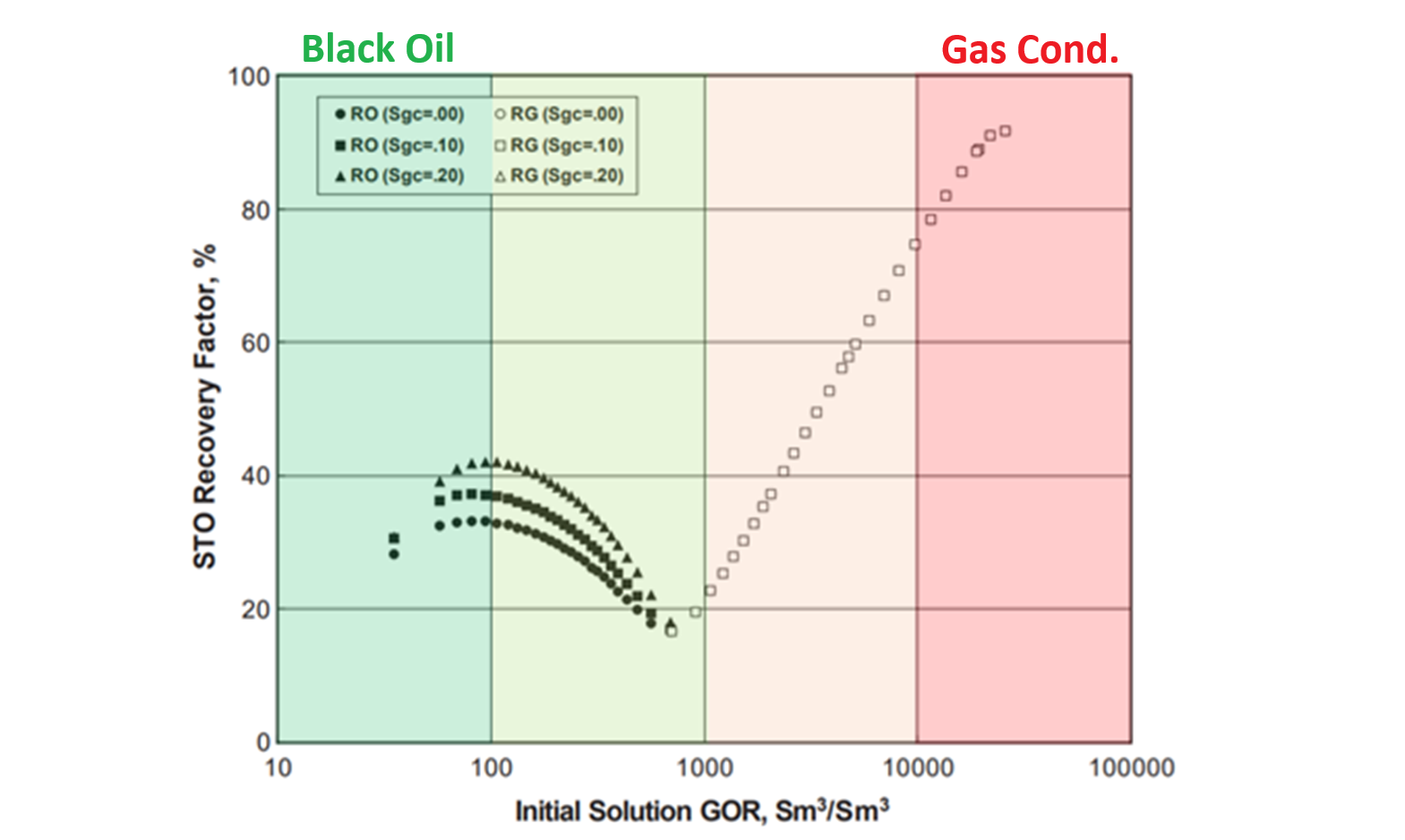
Fun fact
Solution Gas Drive: Around 500-600 scf/STB (~100 Sm3/Sm3) is actually where solution gas drive is the strongest!
5. Forecast
Once the production history is matched, the results can be used to forecast production. In whitson+, the simulation forecast is controlled by pressure (i.e., BHP or WHP). After making any changes to the forecast schedule or toggle, the simulation must be rerun to update the results.
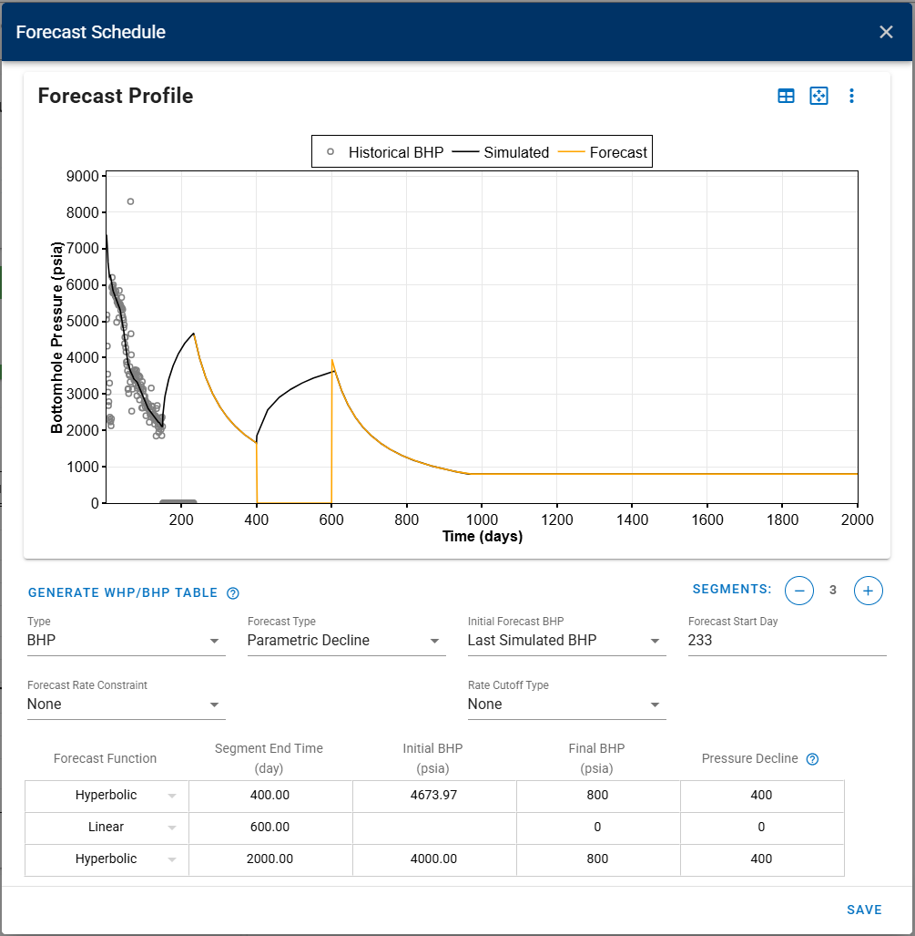
5.1. BHP Forecast Type
whitson+ provides three alternatives in creating BHP forecast:
-
Parametric Decline to set the forecasting function between the input initial and final BHP as hyperbolic or linear based on the input Nominal Pressure Decline in %/yr or psia/d, respectively.
-
Hyperbolic decline: The pressure declines at a constant percentage per year. The daily pressure is calculated as:
where \(X_{hyp,decline}\) is the hyperbolic decline rate in %/yr. -
Linear decline: The pressure declines by a constant value per day. The daily pressure is calculated as:
where \(X_{lin,decline}\) is the linear decline rate in psi/day, kPa/day, or bar/day.
-
-
Constant BHP throughout simulation time.
-
Custom Schedule provided by user in table-wise manner. By default, the first row will be the BHP at the last time step of history matching simulation run.
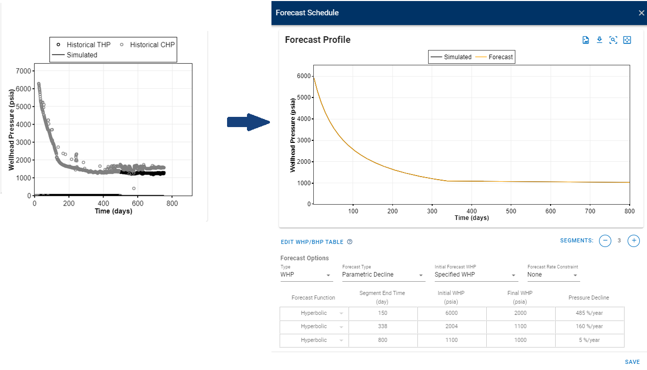
5.2. WHP Forecast Type
whitson+ provides three alternatives in creating WHP forecast:
-
Parametric Decline to set the forecasting function between the input initial and final WHP as hyperbolic or linear based on the input Nominal Pressure Decline in %/yr or psia/d, respectively.
-
Constant WHP throughout simulation time.
-
Custom Schedule provided by user in table-wise manner. By default, the first row will be the WHP at the last time step of history matching simulation run.
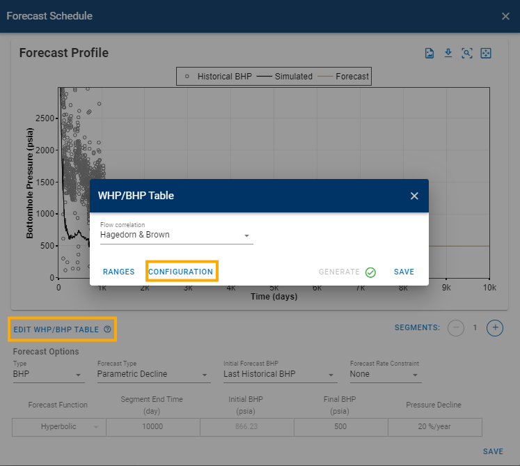
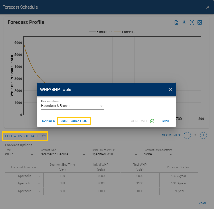
5.3. Edit WHP/BHP Table
The WHP/BHP table is used to:
-
Compute the WHP when forecasting on a BHP profile.
-
Compute the BHP when forecasting on a THP profile.
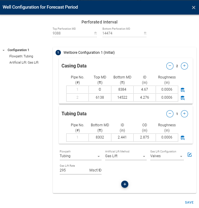
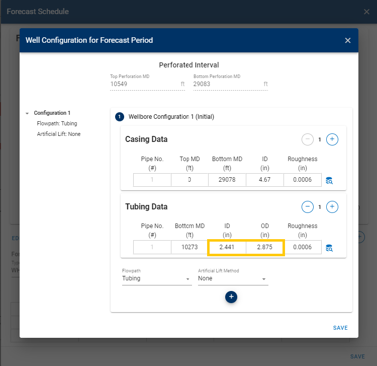
The flow correlation and wellbore configuration are editable for the forecast period, as shown below.
5.4. Forecast Shut-In Periods
Users can simulate cyclical shut-in periods during forecasting to evaluate pressure build-up effects and their impact on future production. This feature is useful for modeling operational pauses, economic shut-ins, or pressure maintenance strategies, helping users understand reservoir behavior during non-producing intervals.
How to model shut-in periods in forecast:
- Navigate to the EDIT FORECAST SCHEDULE.
- Ensure the "Type" is set to BHP, and the "Forecast Type" is Parametric Decline.
- Add new segments for the shut-in segments.
- Configure the shut-in segments settings: "Forecast Function" is Linear with 0 "Pressure Decline".
- After each shut-in segment, add a new flowing segment, allowing the model to simulate pressure drawdown and production.
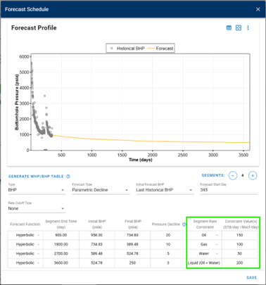
5.5. Segment-based Forecast Constraints
Forecasting accuracy can be improved by applying rate constraints to each segment individually rather than relying on a single well-level constraint
6. Autofit
6.1. How to run Autofit
It is possible to automatically history match a numerical model to historical data with the "Autofit" option. To run the "Autofit",
- Click the AUTOFIT-button to the upper left.
- Select parameters you would like to alter (\(x_f\) and \(k\) are defaults).
- Provide their ranges for each parameter.
- Turn on/off weighting for relevant timeseries (global weighting switch).
- Click AUTOFIT to the lower right.
6.2. Set Weighting Points
In addition to the global weighting switch, you can set different weighting throughout time.
Each timestep can be set to either
| Weight | Description |
|---|---|
| 1 (default) | Assigned to standard data points. |
| 10 | Marks data as high-priority for history matching. |
| 0 | Indicates low-confidence or poor-quality data (effectively ignored in the match). |
What is a weighting factor?
A weighting factor is a numerical parameter that assigns importance to data points during mathematical optimization, here in history matching numerical models to observed data. It helps prioritize or de-prioritize specific data points, optimizing model parameters for a more accurate fit.
6.3. Weighting & Residuals
whitson+ facilitates regression on parameters to minimize the sum of squares of weighted residuals in the context of observed data and corresponding predictions. The objective function in is defined as:
Here, represents the RMS residual error between observed measurement and its corresponding prediction, while is the user-assigned weighting factor for that residual. Ideally, these weighting factors should be inversely proportional to the standard deviations of the residuals. Minimizing in provides the maximum likelihood estimation of the model parameters, assuming independent and normally distributed residuals.
The default weighting factors are 1, while they can also be set to 0 (no importance), and 10 (high importance). Reported is a root-mean-square (RMS) residual defined as:
This metric is related to but is more easily interpreted. The residuals are calculated as relative percentages using the formula:
where is the historical production value, is the simulated value, and is the reference value for observation . The reference value is the nonzero weighted value in the series with the largest magnitude.
6.4. Optimization Algorithm
The optimization algorithm consists of performing Newton steps using a finite-difference calculated Jacobian. The linear system of equations each iteration is
and is solved using Singular Value Decomposition (SVD) of the Jacobian.
6.5. Convergence Criteria
The optimization process terminates based on two primary criteria: solution convergence and iteration limits.
Solution convergence is achieved in one of two ways
- Convergence to minimum when either the SSQ \(\Chi^2\) is driven to 0.0, or if the maximum absolute value of the \(\Delta x\) is less than a specified tolerance
- No significant improvement is made to the solution by continued iteration
The iteration limit is set to 50.
7. Refrac Analysis
A ‘refrac’ or refracturing treatment refers to the process of performing another hydraulic fracturing operation on a well that has already undergone the process in the past.
Typically, you may want to evaluate a refrac that was recently performed on one of the wells. To do that, use the MFMB feature - The workflow is outlined in this section here.
Sometimes, you also want to be able to predict the initial rates and subsequent decline for a refrac that is planned on a well in the future. To do that, use numerical modeling as shown below.
7.1. Workflow for estimating uplift on planned refracs
This section outlines our recommendation for what the simplified workflow could be -
-
History match the target well using BHP as Well Control and resolve a numerical model with high confidence.Then forecast this model to generate a baseline future expectation from the well, under current conditions as shown above in section 4 above.
-
Copy the well (Wells page --> Click the three dots to the right of the well name --> Copy well)
-
On the copy of the well, continue using BHP as Well Control and modify the numerical model to reflect the expectation from the refrac, i.e. -
a. Change the completion - increase the number of fractures (Nf) or fracture half-length (xf) or both.
b. Increasing Nf will primarily accelerate depletion but yeild a higher intial rate.
c. Increasing xf (if we expect a bigger refrac completion) will add additional pore volume
d. Forecast this updated model.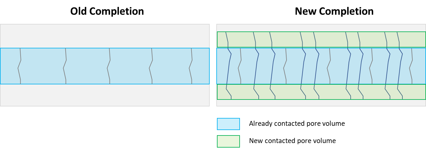
-
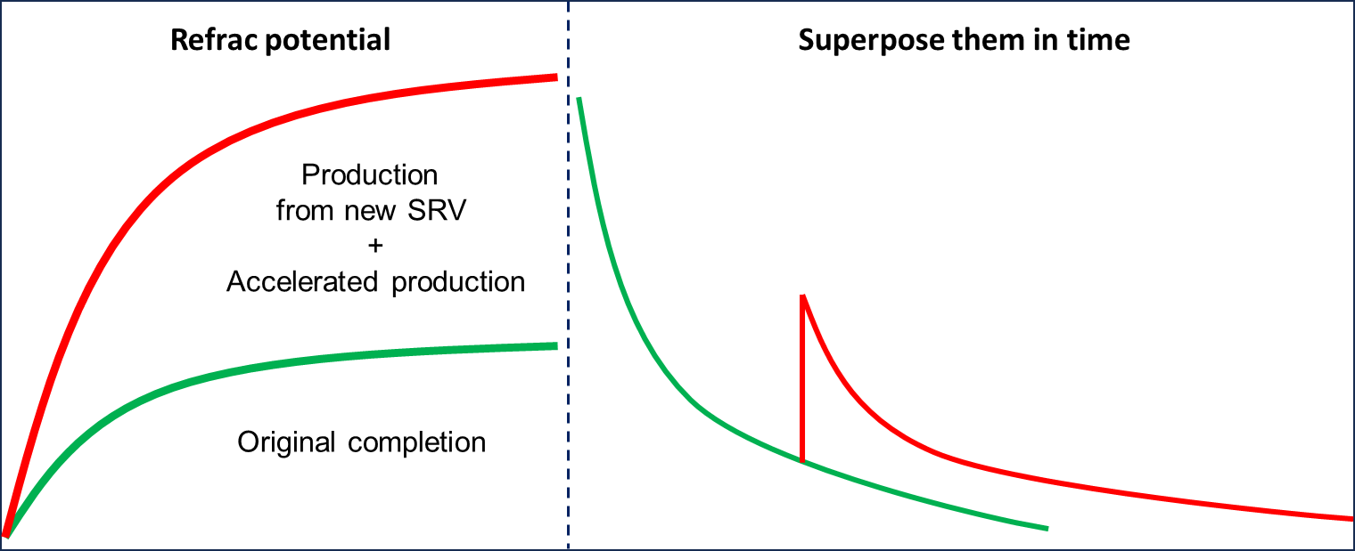
Delta between outcomes of Steps 1 and 2 is the refrac potential of this well.
-
Superpose these resulting rates at the time of refrac to get the uplift expected after refrac
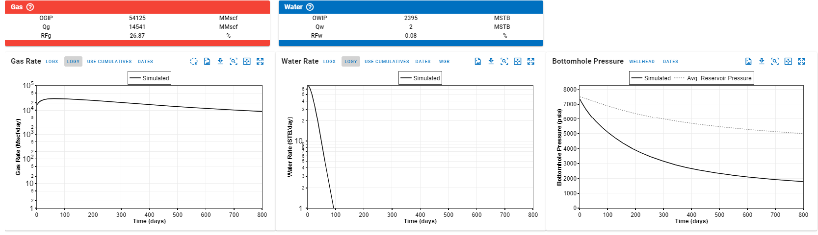
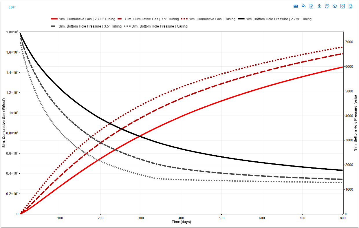
8. Sensitivities on Tubing/Casing Sizes with the Numerical Model
Sensitivity analysis of tubing/casing sizes can be done in the software using tubing tables within the numerical model. This allows imposing a surface pressure constraint.
Tubing tables are only applicable for the forecast period
However, to apply sensitivity analysis to the historical period, a workaround can be employed. This involves creating a new well without historical data and utilizing the forecast section to reproduce the observed surface pressures. The following steps outline the workaround:
- Copy the well: Create a copy of the original well.
- PVT: Initialize PVT
- Remove historical data: Delete the existing production data from the copied well.
-
Match wellhead pressure: Replicate the observed wellhead pressure profile in the forecast profile of the copied well.
-
Modify tubing table: Adjust the configuration of the WHP/BHP table (tubing tables) to analyze the effects of different configurations.
-
Run WHP forecast simulation: Run the numerical model in WHP type for the forecast option.
-
Repeat for other tubing sizes: Create new scenarios and repeat steps 5-6 for each tubing size you want to analyze.
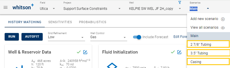
-
Compare results: Use a comparison plot to visualize the results from all the sensitivity run.
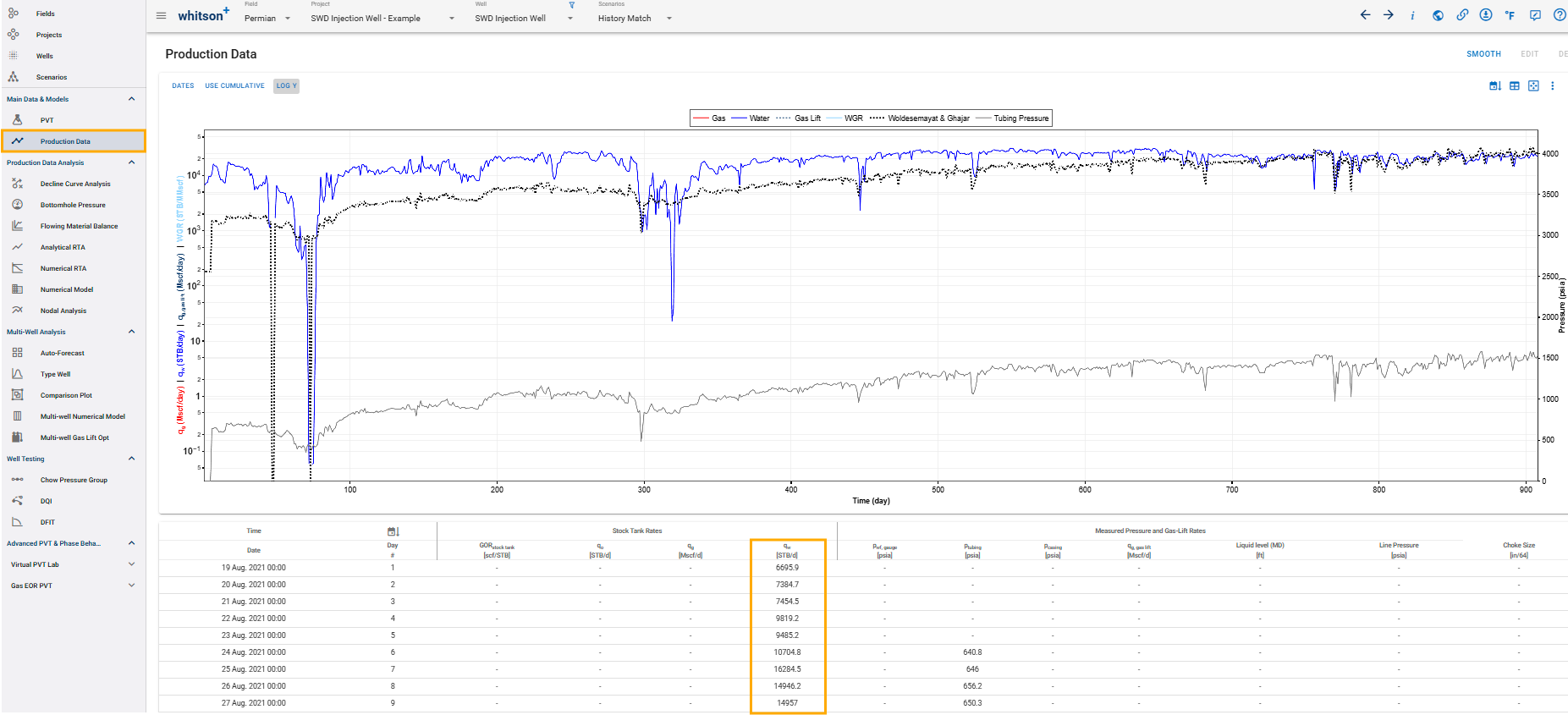
9. Saltwater Disposal Injection Well
9.1. History Matching Workflow
-
Upload the required data for this analysis: water injection rates, tubing/casing pressure, tubing/casing configuration, and well deviation survey. The default wellbore diameter for vertical radial well is 0.5 ft (corresponding to a wellbore radius of 0.25 ft).
Water Injection Rate
The water injection rate must be loaded as 'Water Rate' (no necessary negative values).
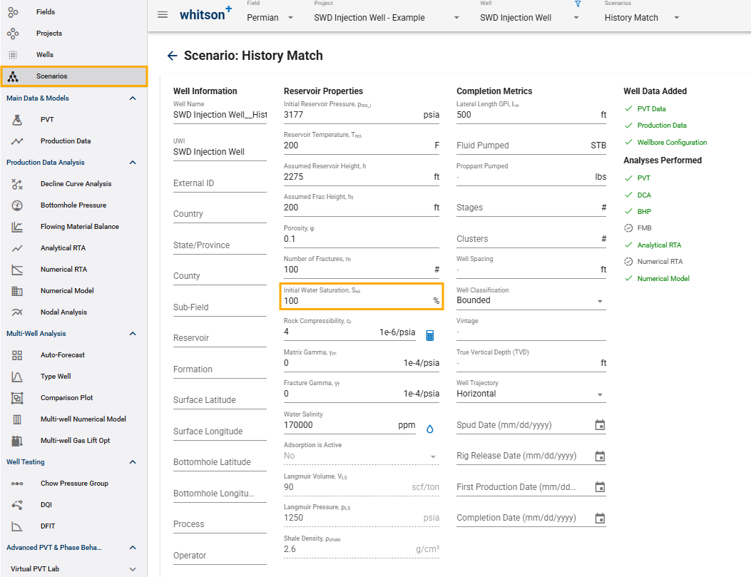
-
Set the initial water saturation (Swi) to 100%.
-
Initialize PVT the default PVT. While the PVT isn't directly relevant to this specific analysis, running this process is a prerequisite for the following modules.
-
To model the bottomhole pressure during an injection process, it is necessary to activate the BHP injection mode. This is done in the Calculation Settings in the Well Data card (see .gif below).
Remember
When enabled, this switch allows to simulate the pressure at the bottom of the wellbore during injection and all uploaded rates will be assumed to be injected rates.
-
To adjust the fluid density in SWD wells is done through water salinity in Water PVT & Viscosity:
-
Numerical Model: History Matching
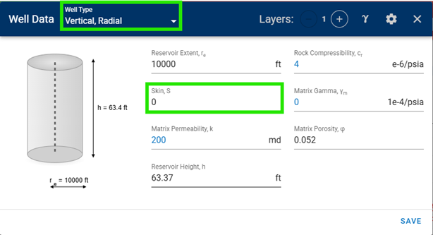
a. In Well & Reservoir Data Card select “Well Type: Vertical, Radial” and input the reservoir properties:
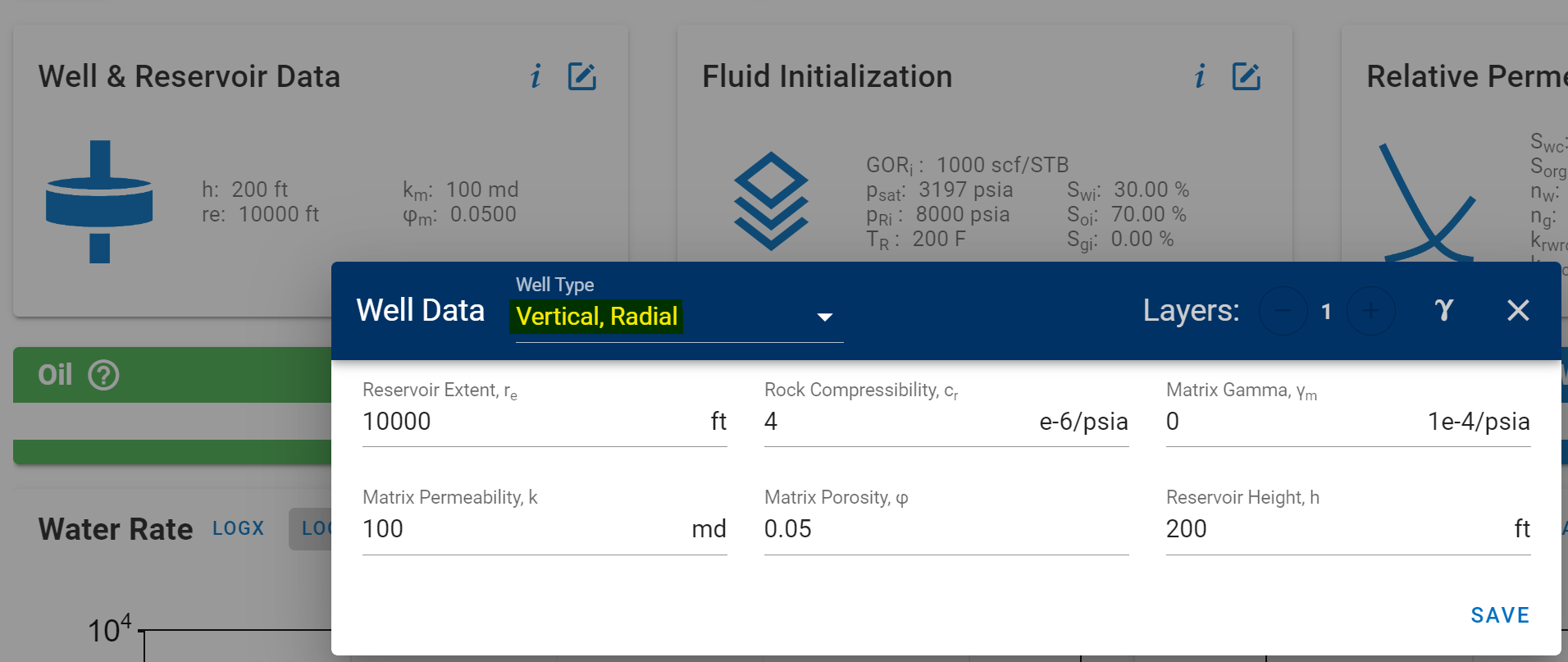
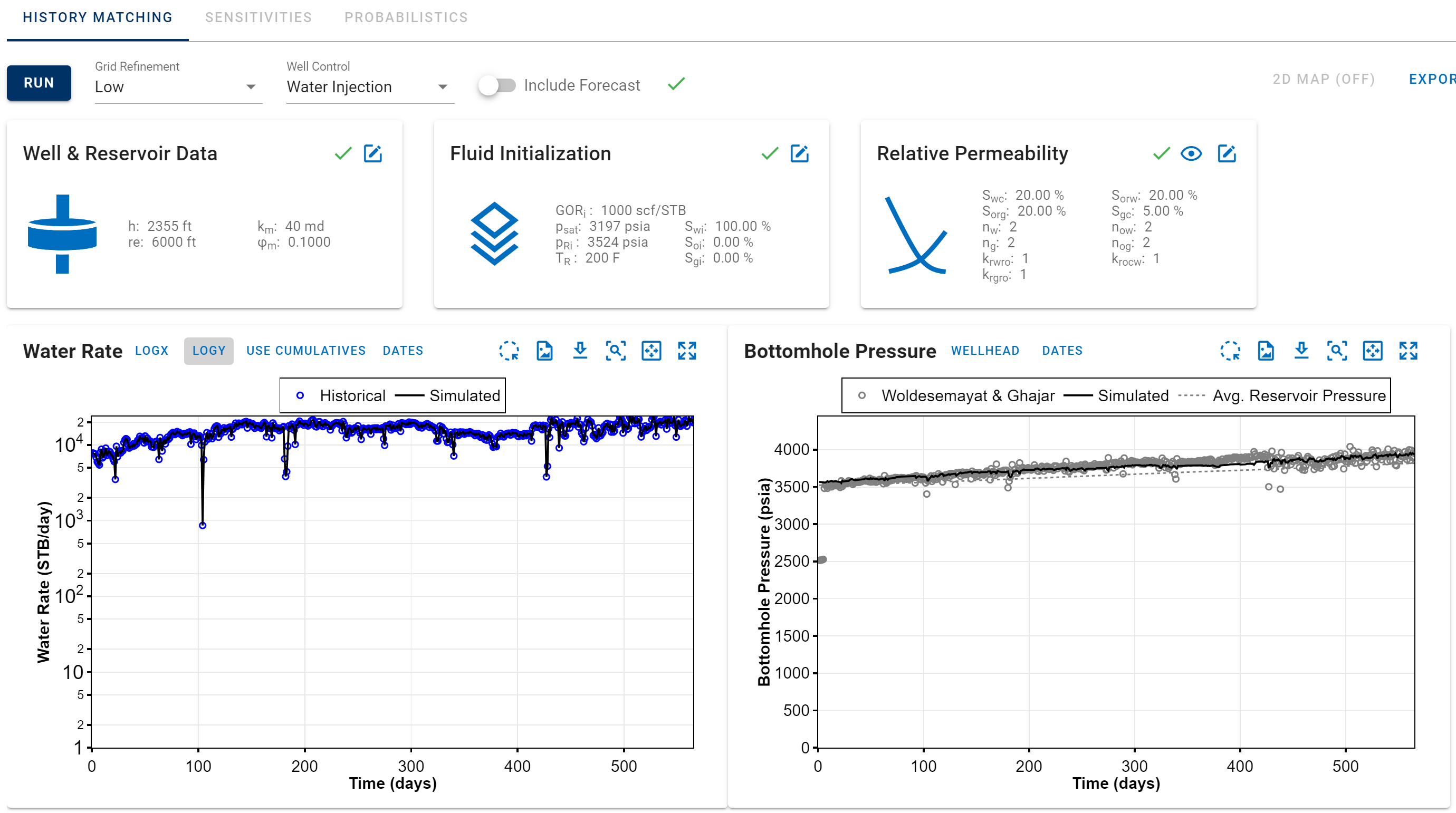
b. Set well control to "Water Injection":

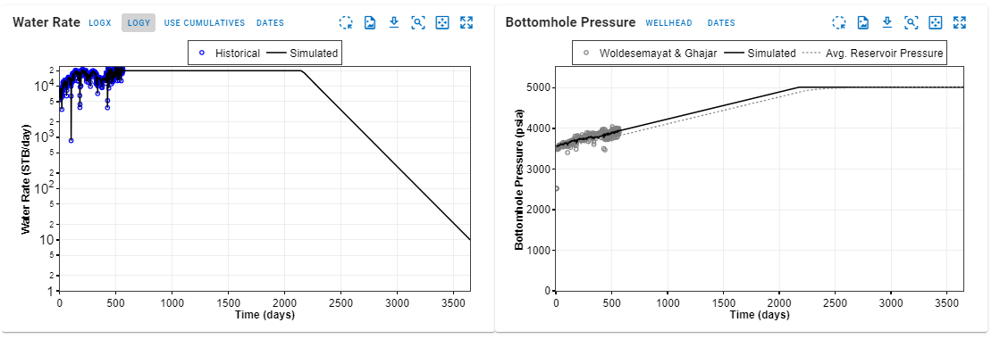
c. Run the numerical model, compare the historical data with the simulated results.
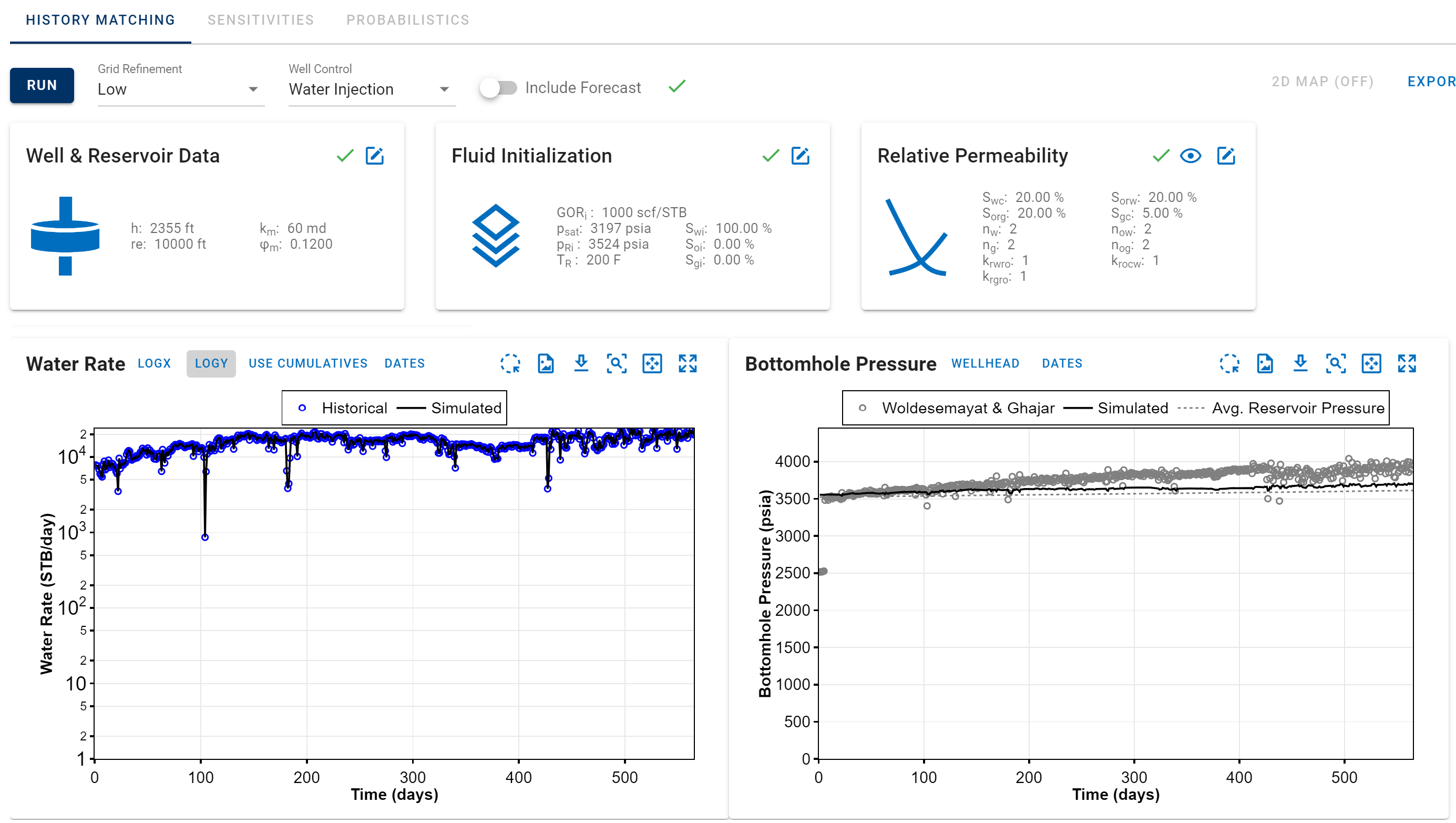
d. Adjust the reservoir properties and any other relevant data as needed to achieve the desired bottomhole pressure.
-
Numerical Model: Forecast
a. Check the box “Include Forecast”.

b. Edit Forecast Schedule

c. Set Forecast Options: Forecast type, initial forecast water and the constraint. And set the Forecast Profile: Forecast end time, constant water.
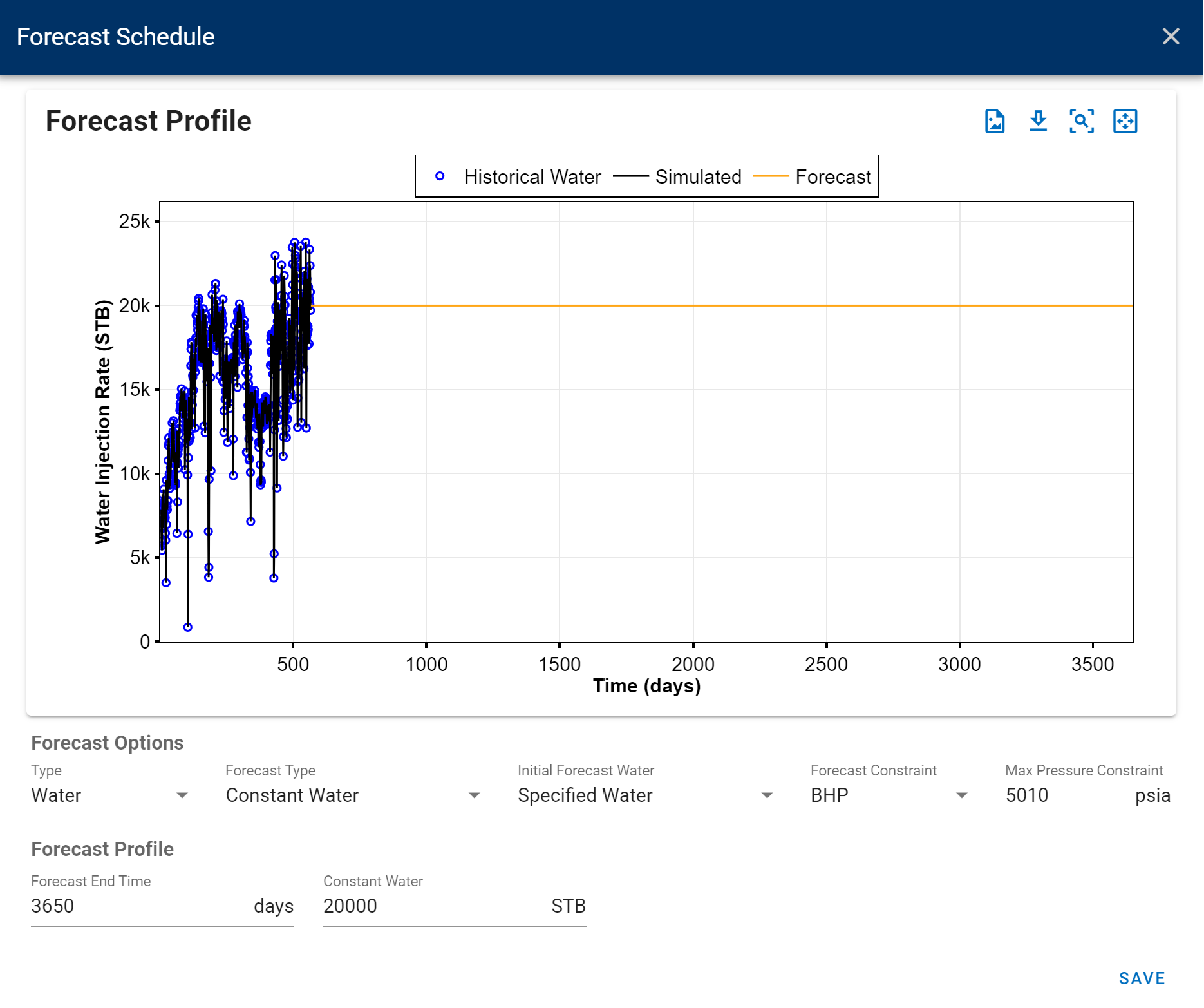
d. Run the simulation.
9.2. Skin Application in the Numerical Model
9.2.1. Positive Skin (Skin > 0)
Positive skin is directly included in the connection factor calculation. This connection factor is then passed to the simulator to compute the well productivity index. In radial geometry, the formula used to calculate the connection factor, , depends on the location of the connecting grid block. When the connection is situated in one of the innermost grid blocks (), it is assumed to lie on the inner boundary of the block. The connection factor is calculated using the followinf formulation:
where:
- is the unit conversion factor (0.001127 in field units, 0.008527 in metric units, 3.6 in lab units)
- is the angle of the segment connecting with the well, in radians. In a Cartesian grid its value is 6.2832 ( ), as the connection is assumed to be in the center of the grid block.
- is the effective permeability times net thickness of the connection. For a vertical well the permeability used here is the geometric mean of the x- and y-direction permeabilities,
- is the block’s outer radius
- is the wellbore radius
- is the skin factor
9.2.2. Negative Skin (Skin < 0)
Applying a negative skin value directly is not physically realistic, because it can result in a negative connection factor. This happens when the effective wellbore radius becomes larger than the grid block’s pressure-equivalent radius. In such cases, the connection transmissibility factor can become extremely large, which may cause convergence issues in the simulation. If the effective wellbore radius exceeds the pressure-equivalent radius, the connection factor turns negative and the simulator will issue an error.
To avoid this, negative skin is handled by modifying the near-wellbore permeability instead of the connection factor. The negative skin value is used to calculate the smallest altered radius that still results in a positive altered permeability. That permeability is then applied uniformly within the altered region around the wellbore. This approach follows Eq. (\ref{eq:skin-hawkins}) in Well Performance by Michael J. Economides. If the specified negative skin is too severe relative to the radial extent, the simulator will stop the run and return an error to prevent invalid calculations.
The additional pressure drop due to the altered zone is obtained by subtracting the bottomhole pressure for the undisturbed permeability case from that of the altered zone case:
Following the formulation introduced by Hawkins (1956), the dimensionless skin factor, , is defined as:
Substituting, the additional pressure drop simplifies to:
You can also find a comparison of different skin values in Analytical and Numerical solution here
9.2.3. Skin Effect Option
When the well type is set to Vertical or Radial, you can enable the Skin Effect option in the Well & Reservoir Data input card. This allows the simulator to account for positive or negative skin in the connection-factor calculation for vertical geometry or radial flow.
9.3. Takeaway Capacity – BHP Sensitivity to Permeability
Understanding takeaway capacity is essential when evaluating water disposal wells. In whitson+ , users can utilize the numerical model to simulate bottomhole pressure (BHP) requirements at various permeability values and injection rates.
The example shown below represents a vertical well with staged water injection rates ranging from 3,000 bbl/d to 8,000 bbl/d. The required BHP to sustain each rate was simulated at permeabilities of 100, 200, 300, 400, and 500 md.
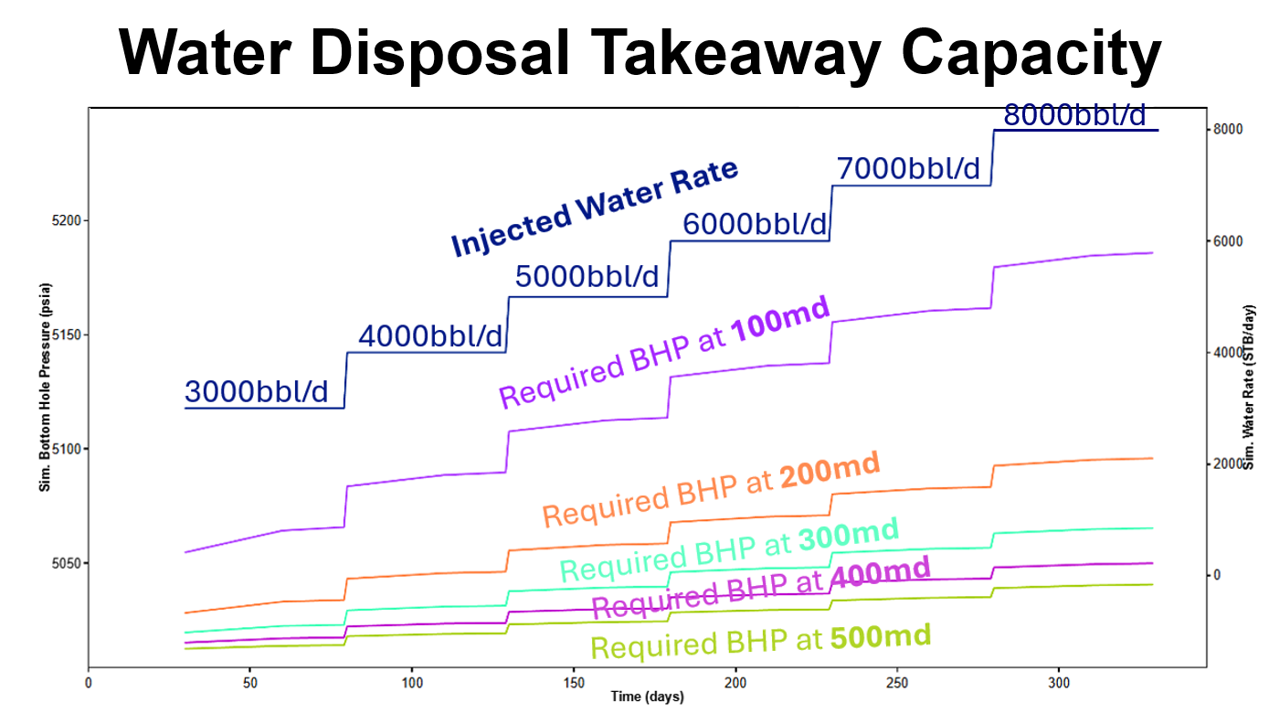
As expected:
-
Lower permeability formations require higher BHP to achieve the same injection rate.
-
Higher permeability formations allow injection at lower BHP.
10. Multi-Fractured Vertical Well
Two types of modeled fractures are supported in Multi-Fractured Vertical Wells:
-
Vertical fractures (default MFVW fracture geometry)
- Single Petrophysical Layer:
- Multiple Petrophysical Layers:
-
Horizontal (pancake) fractures
- Fractures Orthogonal to Z-axis:
10.1. Fracture spacing
The concept of half-fracture spacing used for multi-fractured horizontal wells (MFHW) also applies to MFVW.
- Half-fracture spacing where:
- is net pay (or net perforated height, depending on the well definition)
- is the number of fractures
Because gravitational effects matter in MFVW, the fracture is placed at the center of the fracture spacing. As a result, MFVW models the full fracture spacing (not just ) in the simulation geometry.
10.2. Multi-layer assumptions and runtime impact
When more than one petrophysical layer is introduced, the total number of grid blocks increases with the number of layers:
- 2 layers: roughly 2x the grid blocks
- 3 layers: roughly 3x the grid blocks
- and so on
As the total grid size grows, simulation time can increase sharply, so this option should be used with care.
Multi-layer runs can take longer
Adding layers increases the number of grid blocks and can significantly increase runtime. Consider using fewer layers or a coarser setup first, then refine only if needed.
In the case of multiple petrophysical layers, all fractured layers are assumed to be perforated.
10.3. Modeling fracture height smaller than net pay
In order to make fracture height < net pay in a multi-layer MFVW setup, include a matrix-only layer between fractured layers. This gives the model a clear way to represent unfractured rock between fractured intervals.
Practical setup tip
A simple pattern is: fractured layer, matrix layer, fractured layer (repeat as needed), where the matrix layer represents the unfractured interval.
10.4. Scaling and volume reporting
Volumes in place are calculated based on the simulation model dimensions. A scale factor is then applied before reporting values to the frontend.
- Single-layer MFVW (and cases where symmetry is used): scale factor is
- Multi-petrophysical layer MFVW (fractures modeled explicitly): scale factor is 4 (since the model explicitly represents every fracture and does not need multiplication by )
11. Export Results and Other Options
To date, the production forecast results can be exported in excel format in daily or monthly option, while the dataset can be exported into OPM Flow, Eclipse, and CMG:
- Daily Rates
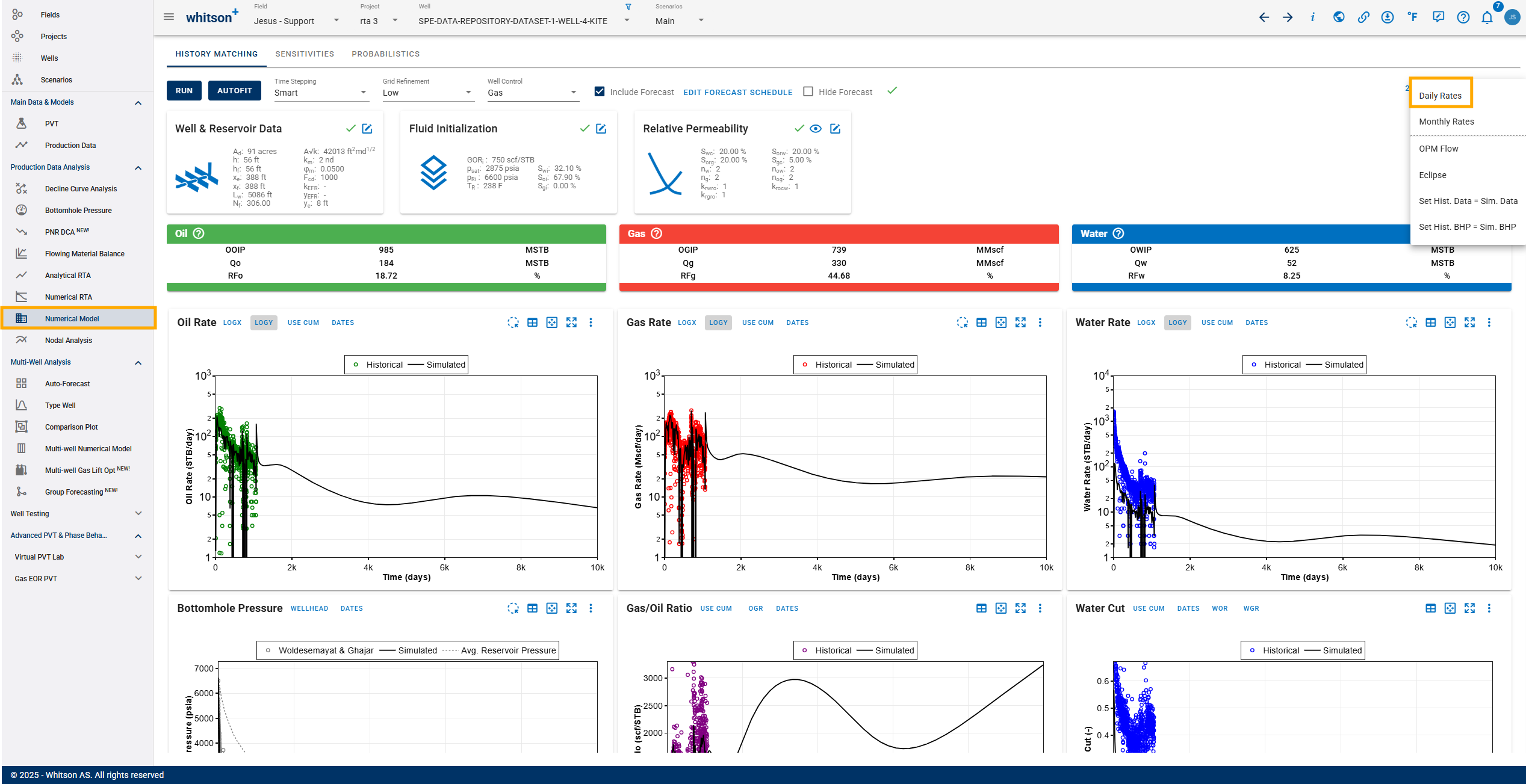
- Monthly Rates
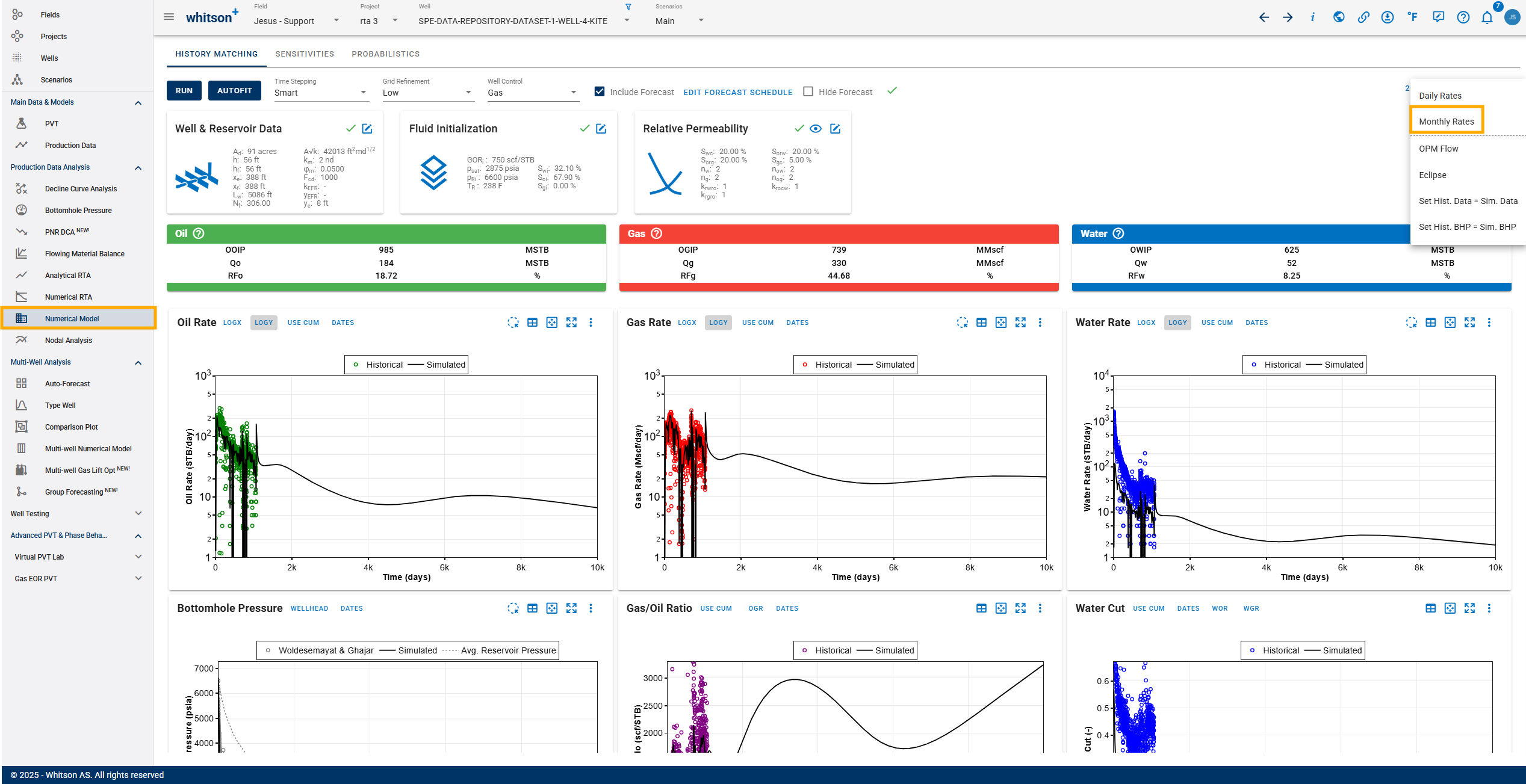
- OPM Flow
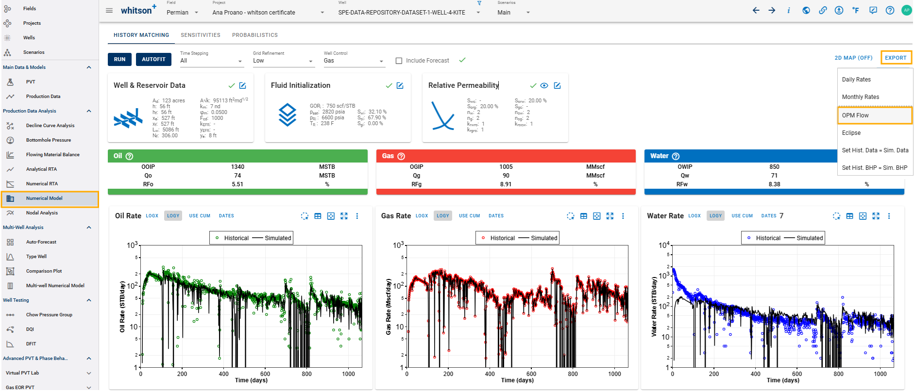
- Eclipse (E100)
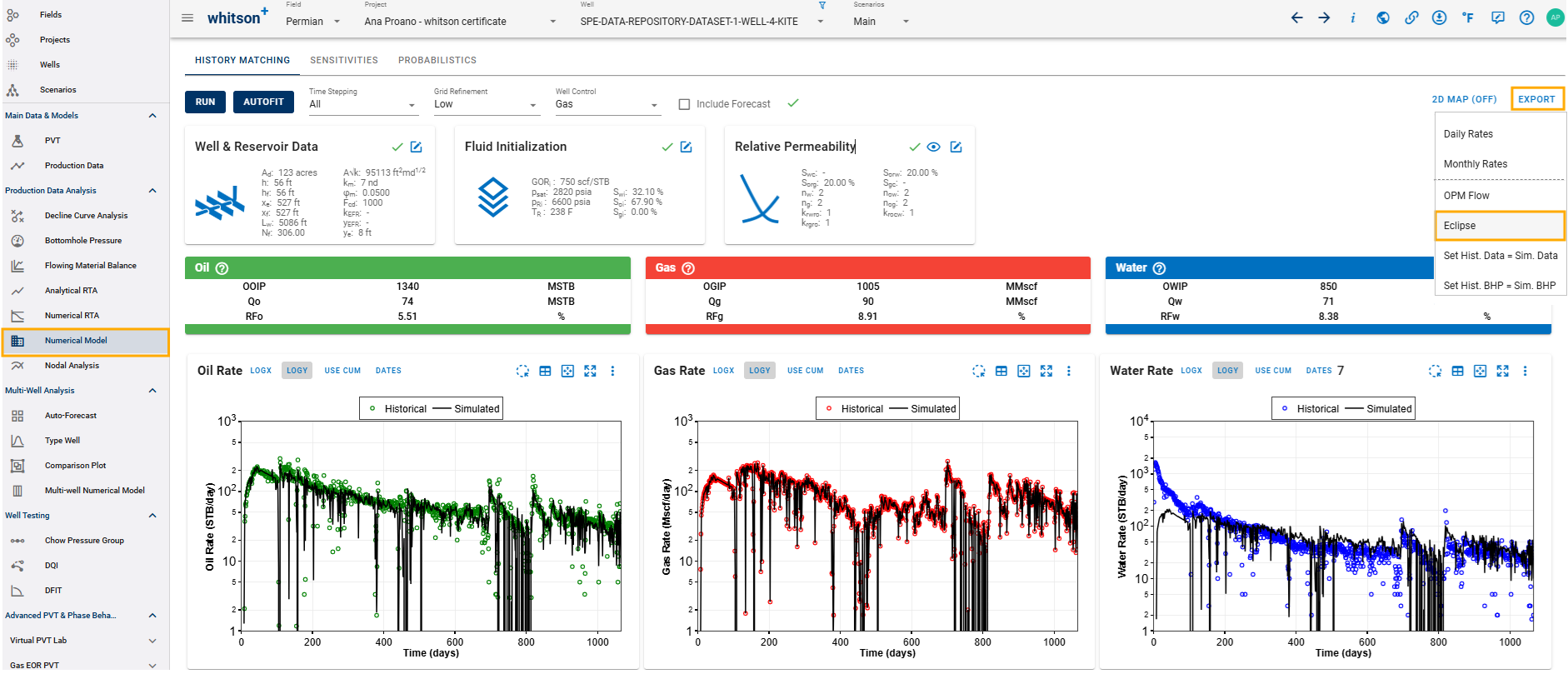
- CMG
Currently, there's no direct export option to CMG. However, you can utilize the ECLIPSE-generated file as an intermediary. This ECLIPSE file can be directly converted into the CMG IMEX format using the CMG converter tool.
As shown in the image below, you simply drag and drop the ECL100 file generated by whitson+ onto the CMG converter.

Let us know, if you'd like us to add another export option for your company. Contact us or use the Send Feedback button at the top right of whitson+.
11.1. Experimental Features
Apart from these exports to Excel, etc., this section also contains the following set of options to export simulated results to update the production data table in whitson+.
- Set Hist. Data = Sim. Data: Updates the entire production data table for the well on whiston+ to replace the actual production rates and pressures with the simulated rates and pressures from the model. Note that the simulated rates and pressures will now replace the actual data here, so the real field production data (if it exists) will be lost.
- Set Hist. BHP = Sim. BHP: Updates only the gauge pressure in the production data table to be replaced with the BHP simulated output from the numerical model - does not replace any rates.
You can even build models first for synthetic wells without any production data, generate simulated output using BHP(synthetic) as well control, and use these options to generate a synthetic production data table, that is still true to the model, given the drawdown. These can be used to build and verify mental models of depletion, flow regimes, what-if analysis for drawdown scenarios and comparison.
11.1.1. Creating Synthetic Wells
Here's a GIF to show you how you can use these features quickly create a synthetic well and use the simulated data with the other features in whitson+ to test them on a simulated reservoir response-
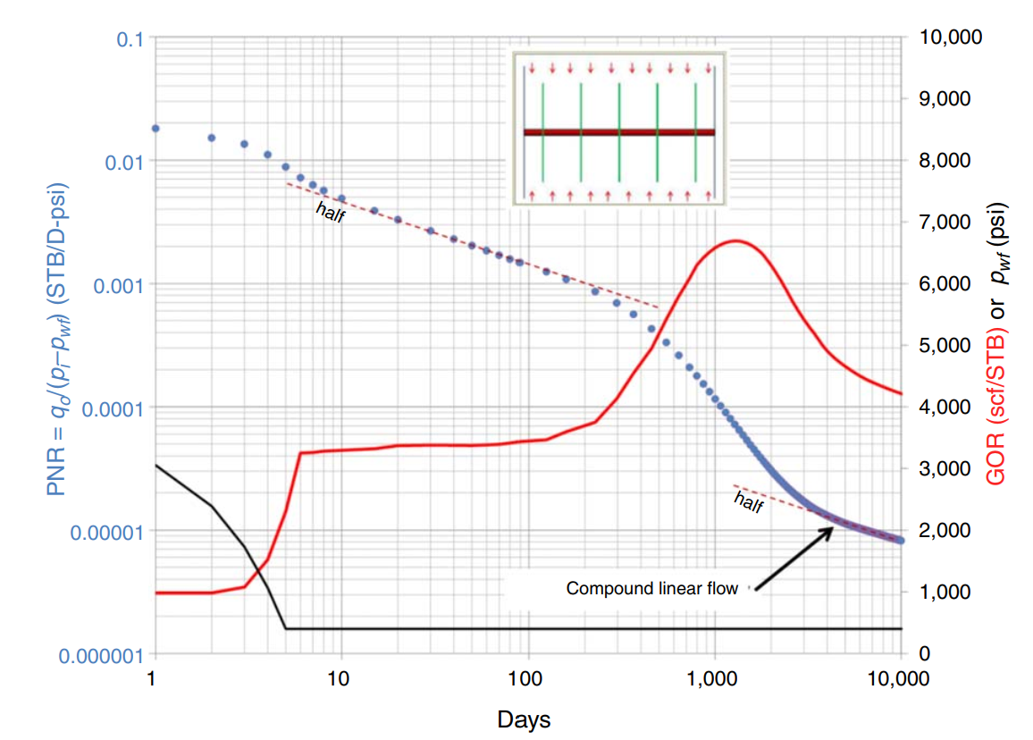
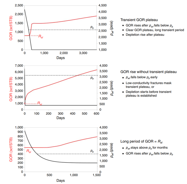
12. Producing GOR in Multifractured Horizontal Wells
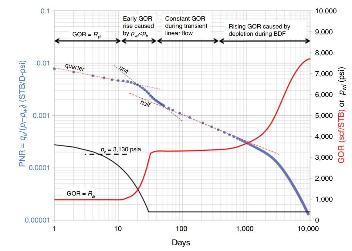
Horizontal wells with hydraulic fractures in tight oil reservoirs how producing GOR behavior that is very different from conventional, higher-permeability reservoirs (Steve Jones, 2016). Observed GOR behavior in tight black-oil reservoirs can be modelled after the following idealized stages throughout history. Some stages might not be visible becuase of the degree of undersaturation, flowing bottomhole pressure schedule, finite conductivity fractures and duration of infinite acting flow period. The stages are
- Stage 1: Early GOR is constant at the initial solution GOR (Rsi) while bottomhole flowing pressure is above the bubblepoint.
- Stage 2: A rise in GOR as bottomhole flowing pressure declines to les than the bubblepoint.
- Stage 3: Transient GOR "plateau", which is characteristic of infinite acting (transient) linear flow.
- Stage 4: A continous rise in GOR during boundary-dominated flow (BDF).
Fundamental differences between infinite acting (IA) flow and boundary dominated flow (BDF), and the associated dependence of GOR on flowing bottomhole pressure, are important to understand. During IA (transient) linear flow, the GOR response changes in flowing bottomhole pressure is independent of the permeabilty for infinite-conductivity fractures, but not for finite-conductivity fractures.
Practical observations are;
- Knowing Rsi and the trasnient-GOR-plateau level in an areac an help one interpret where a well is in its GOR history.
- Classical RTA diagnostic plots are altered by rising GOR, and sometimes show an early init slope.
- During boundary-dominated flow, GOR is more a function of cumulative production than of time, but also recover oil more quikcly.
- If compound linear flow develops, GOR can decline late in the well life.
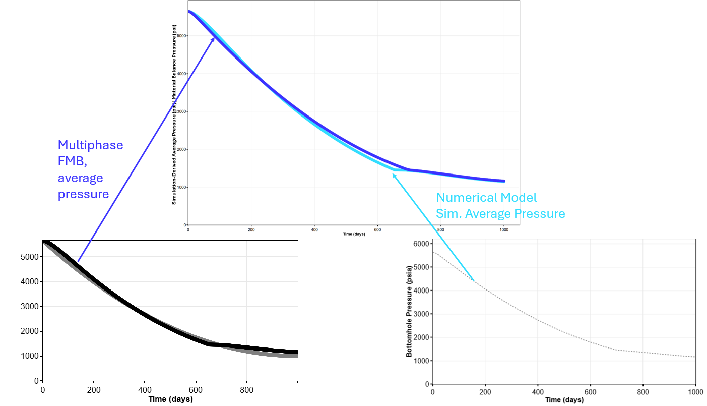
13. Simulation vs. FMB Average Pressure
There is an important distinction between the average reservoir pressure calculated from a numerical simulation model and the material balance pressure back-calculated by FMB.
The simulation-derived average pressure is calculated from the pressure distribution across the grid cells using the averaging or weighting method defined by the simulator, such as pore-volume or hydrocarbon-pore-volume weighting.
In contrast, the FMB average pressure represents the equivalent pressure of a single, well-mixed tank containing the same total fluid mass. It is obtained from the material balance relationship and accounts for pressure-dependent fluid properties and compressibility, including the gas behavior.
The two pressure estimates are equal only when the reservoir behaves as a sufficiently uniform tank with negligible pressure and composition gradients. In real reservoirs, pressure depletion, multiphase behavior, and compositional variation can cause the two values to differ. These differences may become particularly noticeable during transient flow, pressure buildup, or shut-in periods.
References
[2] Open Porous Media. 2023. OPM Flow Reference Manual, Version 2023-04. Oslo, Norway: OPM.