Reservoir Simulation - Probabilistics

This module enables users to perform probabilistic analysis on one or more variables at once.

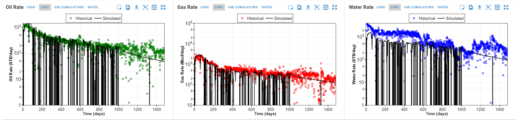
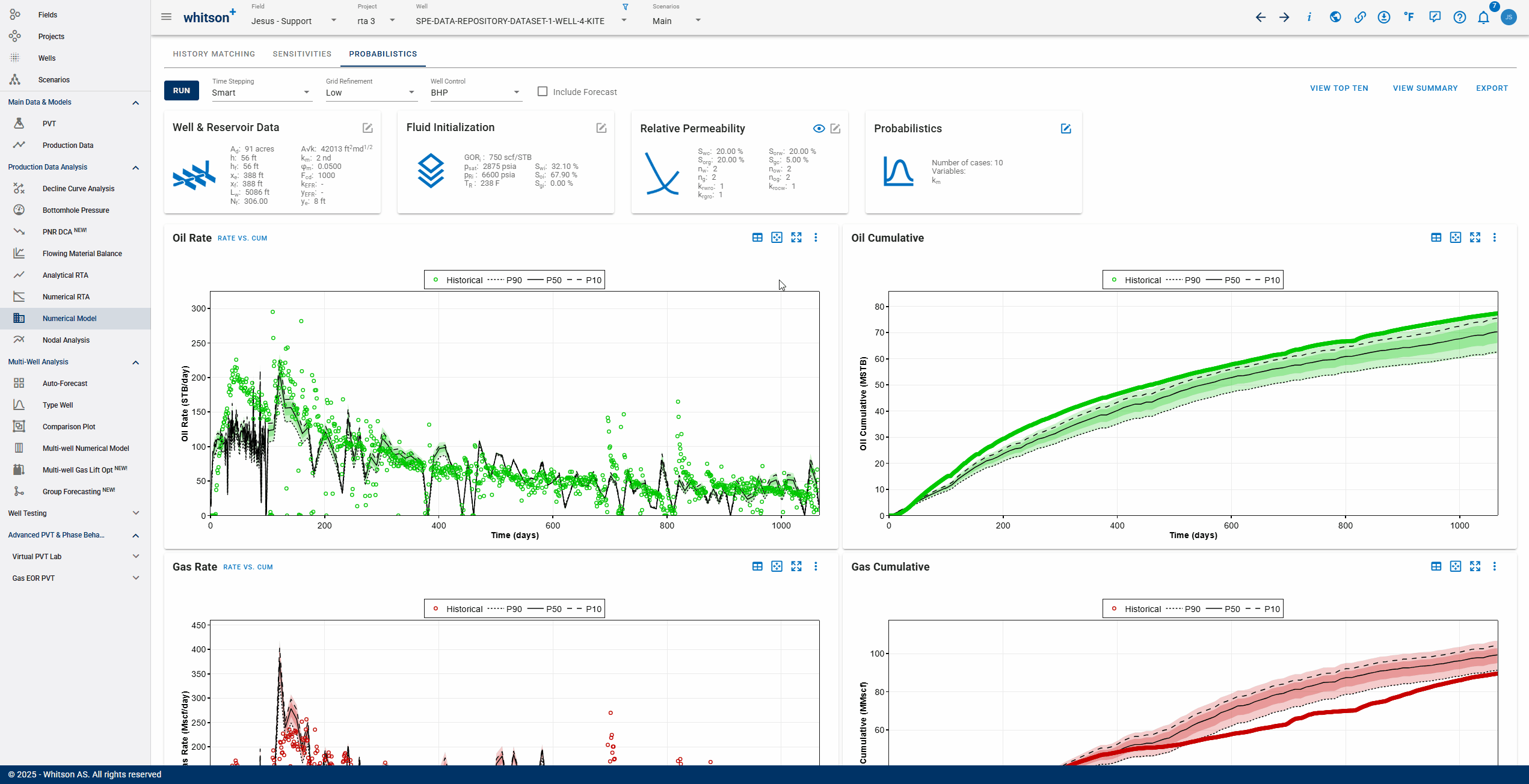
As shown in the GIF below, the probabilistic feature generates simulation results for chosen variables by repeatedly sampling the selected distributions for these variables and rerunning the Numerical Model as many times as the specified number of cases. Results are first sorted by error to exclude cases above the error threshold; only the qualified cases are then used to compute the P90, P50, and P10 and the flowing confidence intervals (shaded areas) in the displayed plots and summary results table.

At least one variable is required to perform this analysis. The number of cases can be set between a minimum of 1 and a maximum of 1000.

There are five distribution types with different inputs required:

Distribution Type	Required Inputs
Uniform	Minimum and maximum value
Triangular	Minimum, peak, and maximum value
Normal	Minimum (P90), maximum (P10), mean value, and standard deviation
Log-Normal	Minimum (P90), maximum (P10), mean value, and standard deviation
Autofit	Minimum bound and maximum bound

Distribution Type - Autofit

The Autofit option performs a tuning process for each realization, similar to Automatic Parameter Estimation (APE). For every sampled set of uncertain parameters, any parameter assigned the Autofit distribution type is automatically adjusted to achieve the best match to the historical data.

For example, if fracture half-length ($x_f$) is sampled from a distribution and permeability ($k$) is set to Autofit, the software will tune $k$ for each sampled $x_f$ before running the final realization.

This approach enables multiple realizations to achieve a similar LFP while representing different combinations of reservoir properties and Original Fluids in Place (OFIP).

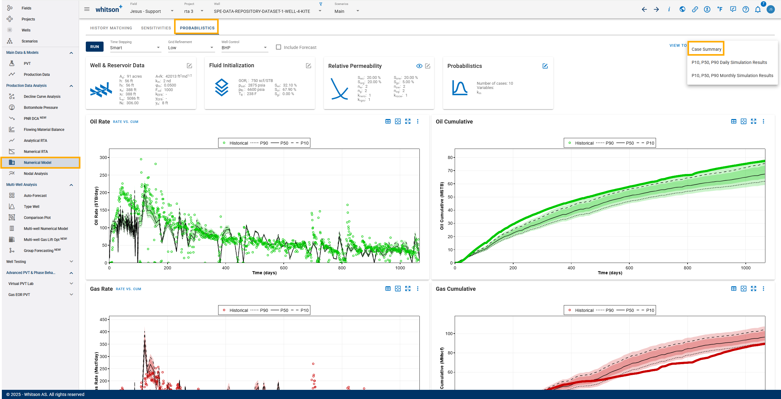
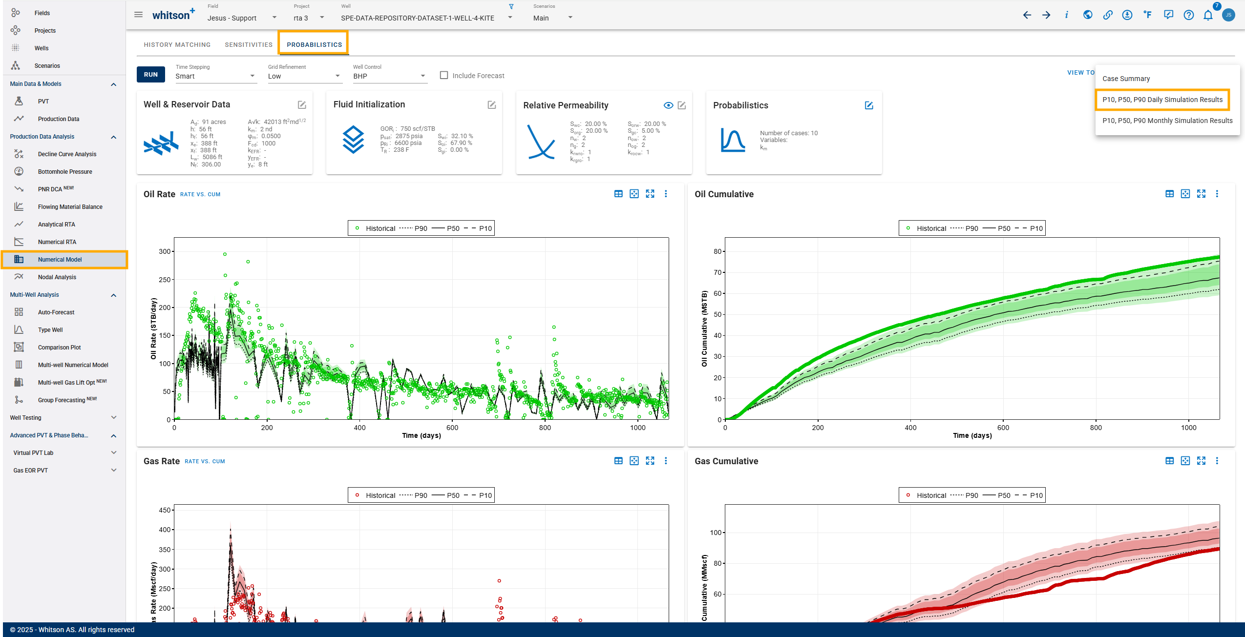
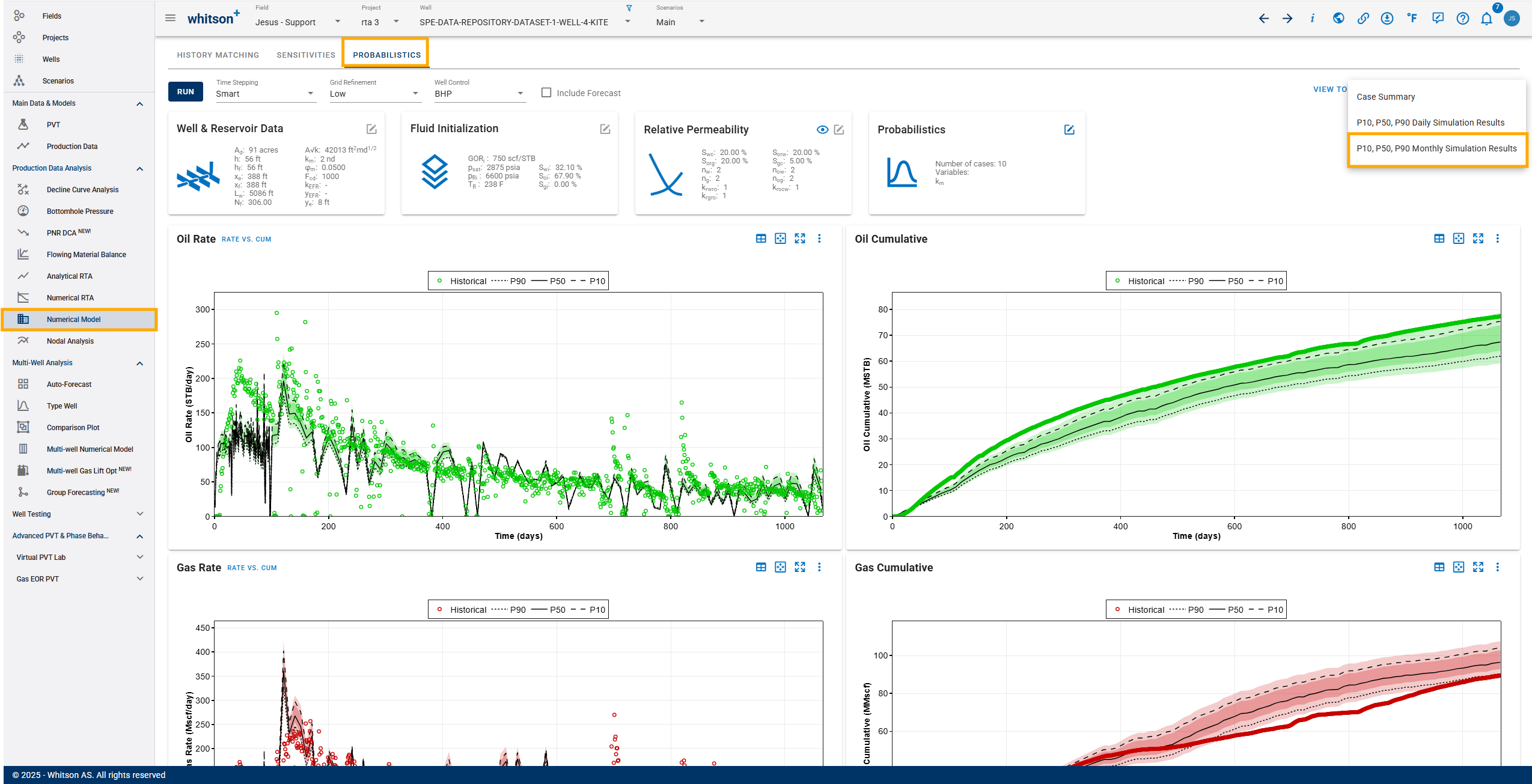
The "View Summary" button shows the summary of P90, P50, P10, mean, and standard deviation of the variables as numeric values. You can also export the summary and/or the simulated results by clicking the "Export" button.

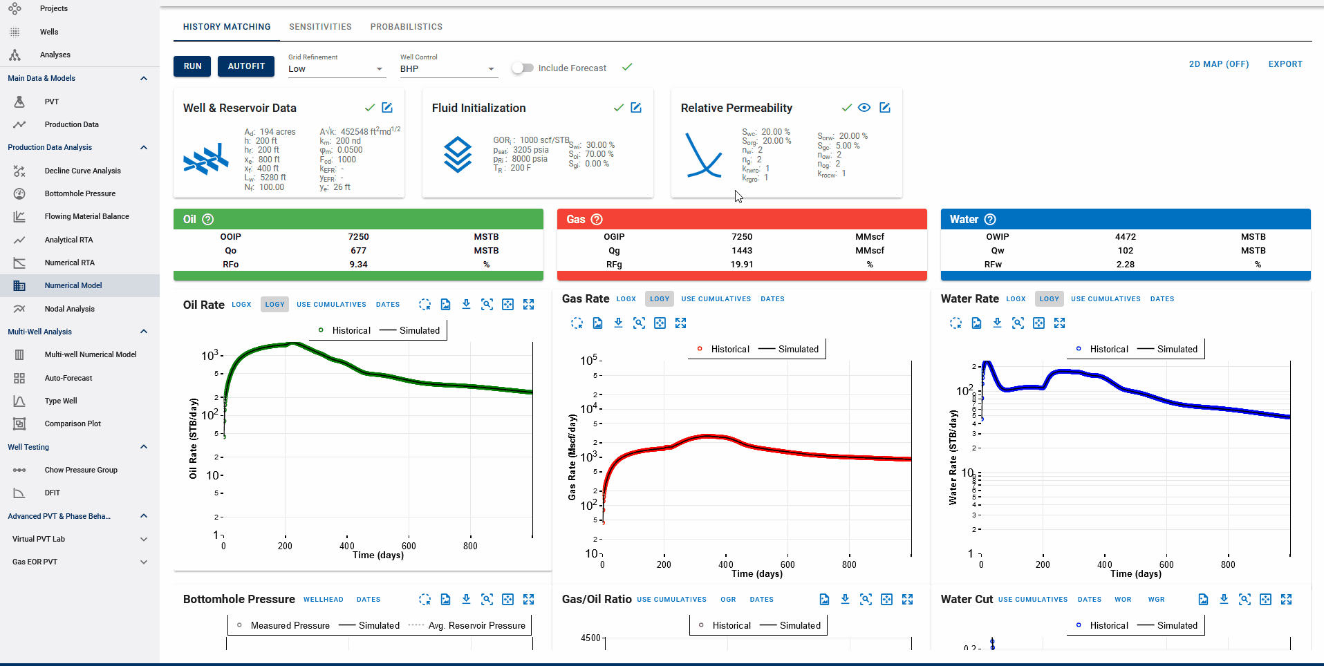
The Numerical Model section includes the following toggles:

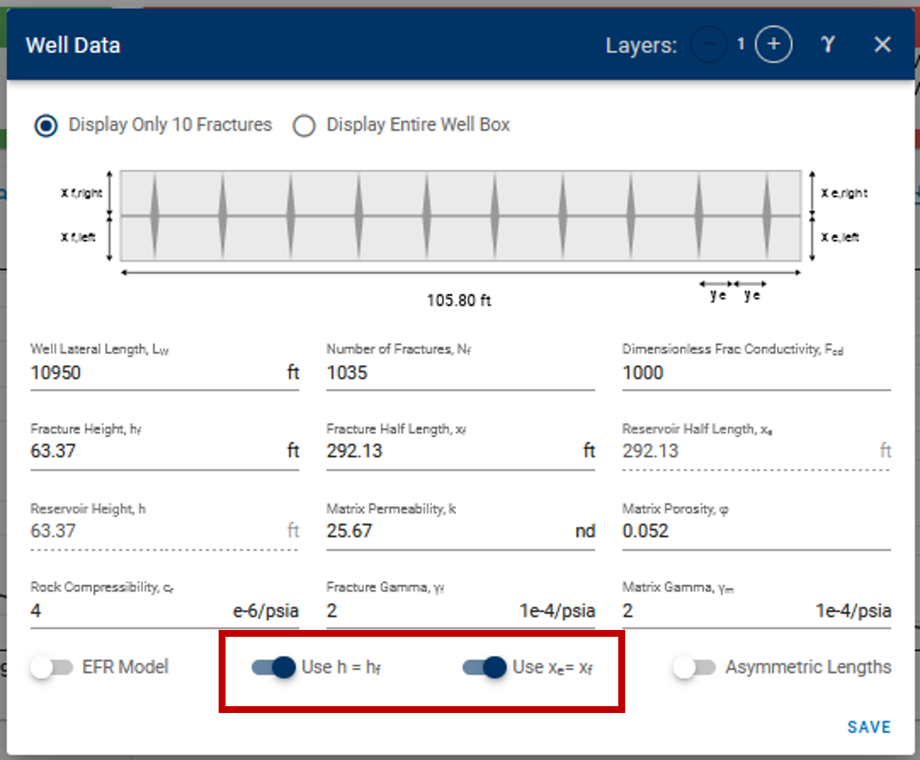
Toggles for h and x_e in Numerical Model settings

When these toggles are switched on, the reservoir height and reservoir half-length are enforced to be equal to fracture height ($h_f$) and fracture half-length ($x_f$) in all simulations — this includes simulation calls via sensitivities and probabilistics.

The default behavior in the probabilistics feature when running probabilistics with $x_e$ (Reservoir half-length) and $x_f$ (Fracture half-length):

1. If $x_e = x_f$ in the model (toggle is on), any specified $x_e$ values are ignored for the given $x_f$; $x_e$ is enforced to equal $x_f$ in the probabilistics case. If $x_f$ is not provided, the base-case $x_f$ is set to $x_e$.
2. If $x_e \ne x_f$ (toggle is off), the specified values of $x_e$ are used; if they are blank, the base-case $x_e$ is used.

Sensitivities and probabilistics cannot override these toggles. To freely adjust $x_e$ and $h$, go to the History Matching section, turn off these toggles on the Numerical Model card, and click Save before running sensitivities. Similar behavior applies for the other pair of variables — $h_f$ and $h$.

Invalid cases

A sampled case is marked as invalid if $x_f > x_e$ or $h_f > h$. Invalid cases are excluded from the valid case count and will not be included in the P90, P50, and P10 results. If you see invalid cases, tighten the parameter bounds so $x_f \le x_e$ and $h_f \le h$.

1. Definition of P10, P50, P90

First, cases are ordered/ranked by cumulative production at the end of history.

• Dry gas and wet gas are ranked by cumulative gas production at the end of history.
• Black oils, volatile oils, near-critical fluids and gas condensates are ranked by cumulative oil production at the end of history.

In the software, the P10 case is defined as the 10th-percentile (best-case) scenario. Similarly, P90 is the 90th-percentile best case, and P50 is the median.

Why do we do it like this?

We want the P10 case of gas to match the P10 case of water (and oil when relevant).

If we assumed a normal distribution at every point and used rates to calculate the standard deviation at each point to define the P10 case for each plot, the P10 stems of gas, water, and oil would have no physical connection. This would not make sense.

However, a normal distribution on every point (or a flowing confidence interval) provides a lot of insight as well. The colored area is meant to visualize this:

• The middle of the dark area is the average.
• The edges of the dark area are one standard deviation from the mean.
• The edges of the light-colored area are two standard deviations from the mean.

This means: if you run a new case with inputs inside the boundaries you have set, there is approximately a 95% probability that the simulation will fall within the entire colored area (this is a rough estimate because covariances are not accounted for).

Summary: The P10, P50, and P90 cases correspond to the same physical simulations in every plot. The colored areas show the 1-sigma and 2-sigma confidence intervals for a new simulation.

2. Error Calculation

whitson⁺ facilitates regression on parameters to minimize the sum of squares of weighted residuals in the context of observed data and corresponding predictions. The objective function in is defined as:

$$\begin{equation} \chi^2 = \sum_{i=1}^{N} (r_i w_i)^2 \end{equation}$$

Here, $r_i$ represents the RMS residual error between observed measurement $i$ and its corresponding prediction, while $w_i$ is the user-assigned weighting factor for that residual. Ideally, these weighting factors should be inversely proportional to the standard deviations of the residuals. Minimizing $\chi^2$ in provides the maximum likelihood estimation of the model parameters, assuming independent and normally distributed residuals.

The default weighting factors are 1, while they can also be set to 0 (no importance), and 10 (high importance). Reported is a root-mean-square (RMS) residual defined as:

$$\begin{equation} \bar{r} = \sqrt{\frac{\chi^2}{\sum_{i=1}^{N} (w_i)^2}} \end{equation}$$

This metric is related to $\chi^2$ but is more easily interpreted. The residuals are calculated as relative percentages using the formula:

$$\begin{equation} r_i = \frac{100(y_{i,\text{hist}} - y_{i,\text{sim}})}{y_{i,\text{ref}}} \end{equation}$$

where $y_{i,\text{hist}}$ is the historical production value, $y_{i,\text{sim}}$ is the simulated value, and $y_{i,\text{ref}}$ is the reference value for observation $i$. The reference value is the nonzero weighted value in the series with the largest magnitude.

3. Running Probabilistics - Targets, Objectives, Weights and Error Thresholds

In the Numerical Model - Probabilistics view, click on the Edit button on the probabilistics card. This opens a dialog box for probabilistic case settings and results are generated with two simple steps -

1. Select Variables - Choose from a range of available variables to run probabilistic simulations.
2. Set Limits - Choose the number of cases to run and set up a distribution (from the types above) for each chosen variable to sample values from.

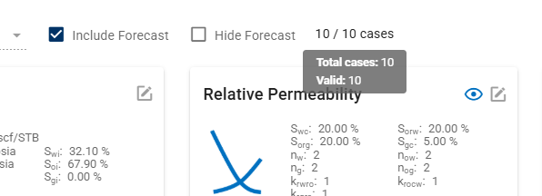
3.1. Weight Factors

It controls which streams are included in the error calculation. A stream (oil rate, gas rate, water rate, or BHP) must be turned on to be included in the objective function and turned off to be excluded. An optional error threshold can be used to exclude poor matches, where any realization with an error above the specified threshold is excluded from the P90, P50, and P10 calculations.

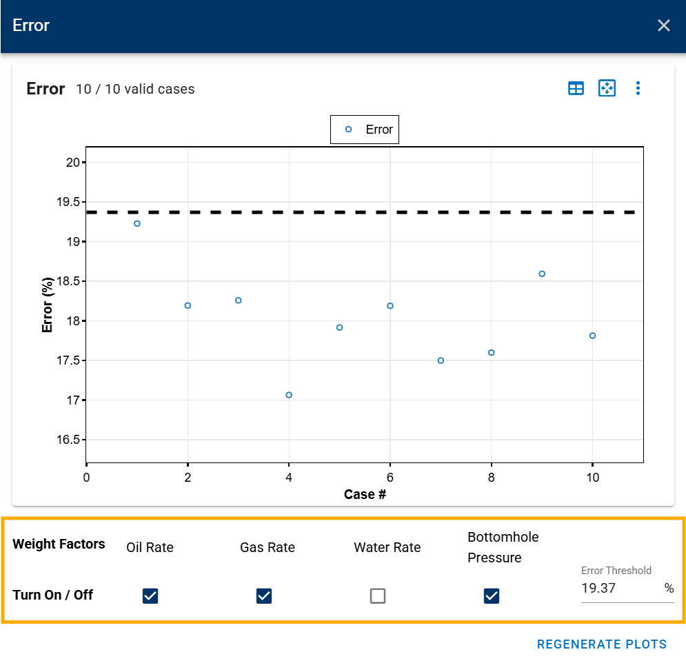
Weight factors used in Numerical Model - History Matching and Probabilistics

💡The RMS error for each probabilistic realization is calculated using the same weighting applied in the History Matching module. Data points marked as Included with the Spray Filter contribute to the error calculation, while data points marked as Excluded are ignored.

In addition, only streams that are turned on in the objective function are included in the total RMS error calculation. If a stream is turned off, all of its data points are assigned a weight of 0, and the stream is excluded from the RMS error calculation for that realization.

4. How to Handle Simulation of Different pRi and GORi?

The black-oil PVT table is always generated in whitsonʳˢ from initial composition ($z_{i}$), reservoir temperature ($T_{R}$), equation of state (EOS), and surface process configuration. The black-oil PVT table is always regenerated locally at runtime, taking only a fraction of a second. This approach ensures flexibility and avoids delays previously encountered when downloading pre-generated BOT files from the cloud.

Current handling for variations in initial reservoir pressure ($p_{Ri}$) and initial GOR ($GOR_{i}$):

The black-oil PVT table is primarily a function of $GOR_{i}$ (through $z_{i}$) and $T_{R}$. The $p_{Ri}$ is used to initialize the fluid as either single-phase or two-phase. This parameter is not a direct input for generating the black-oil PVT table but is used during extrapolation to help avoid numerical instabilities (for example, negative compressibility). Therefore, the extrapolated part of the black-oil PVT table (affected by $p_{Ri}$) is typically outside the region used in simulations and should not materially impact the quality of the results.

• Variations in $p_{Ri}$ with fixed $GOR_{i}$

  When $GOR_{i}$ is held constant, the same $z_{i}$ is used across all cases. Varying $p_{Ri}$ influences the initialization of the fluid system:

  • If $p_{Ri}$ ≥ $p_{sat,i}$, the fluid initializes as single-phase.
  • If $p_{Ri}$ ≤ $p_{sat,i}$, the fluid initializes as two-phase.

  Effects of Varying $p_{Ri}$ with Fixed $GOR_{i}$

  If you compare the files of two History Matching cases with same $GOR_{i}$, but different $p_{Ri}$, there may also be some differences in the extrapolated part of the black-oil PVT table, but that should not impact the simulations.

• Variations in $GOR_{i}$ with fixed $p_{Ri}$

  Changing the $GOR_{i}$ is equivalent to altering the $z_{i}$. For each case, the black-oil PVT table will be generated using a different composition. A new composition ($z_{i}^{*}$) is generated by taking the original $z_{i}$ obtained from Fluid Definition and recombining it to match the specified $GOR_{i}$. A new BOT is then constructed based on $z_{i}^{*}$ and used in the simulation.

• Variations in both $p_{Ri}$ and $GOR_{i}$

  Both effects described in previous points are applied simultaneously.

5. Forecast

Once the variables have been chosen and the model has been run, the results can be used to forecast production. By clicking the "Include Forecast" button, you can append the forecast to the data. However, any edits to the forecast schedule must be made in the History Matching section, and the simulation must be rerun after making changes or when toggling forecast inclusion on or off.

6. Export

Probabilistic results can be exported in Excel format, with daily or monthly options. You can also export a case summary.

• Case Summary

  
  

• P10, P50, P90 Daily Simulations Results

  
  

• P10, P50, P90 Monthly Simulation Results