Classical RTA
1. Theory
There have been many studies showing that infinite acting, linear flow is the dominant flow regime in multifractured horizontal wells for tight unconventional reservoirs. The most common production analysis of linear flow was first introduced by Wattenbarger et al. in 1998. They proposed analytical solutions for both constant rate and constant pressure. In reality, rates and pressures change simultaneously. To account for that, the principle of superposition is applied.
In 1993, Palacio and Blasingame introduced the concept of material balance time (MBT). Material balance time
- is a superposition time function.
- converts variable rate data into an equivalent constant rate solution.
- is rigorous for a boundary-dominated flow regime.
- works well for transient data, but is only an approximation (errors can be up to 20% for linear flow).
In the whitson+ classical RTA module, material balance time is the default time function. Therefore, the theory for the constant rate solution is emphasized in this part of the manual. On the other hand, there is an option to use the constant pressure solution by selecting "Real Time" as a function of time, as presented here.
The purpose of conducting this analysis is to determine the linear flow parameters (LFP=) and drainage volume by interpreting production data. Using Arps' equation with respect to the end-of-linear-flow time , a production forecast can be made.
1.1. Assumptions
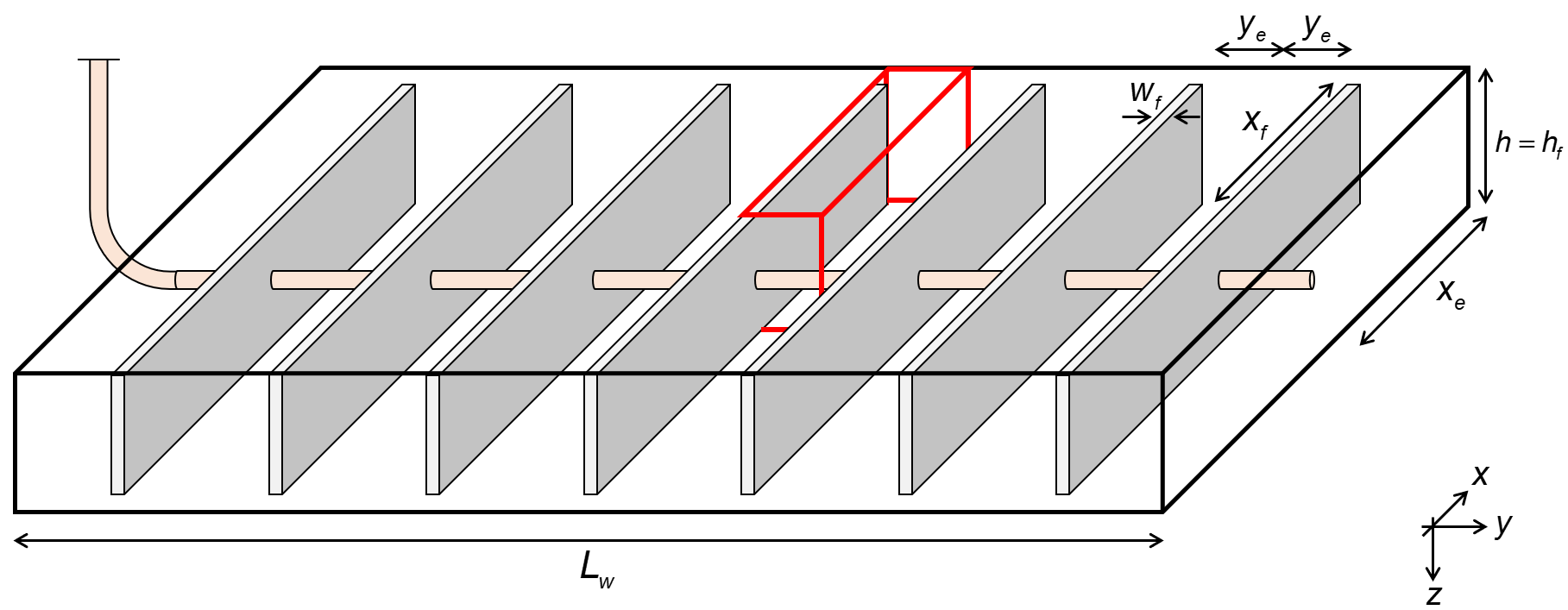
Fig. 1: Wellbox model
Fig. 1 shows the geometry of the well used as a base assumption of these analyses. The fracture is assumed to have infinite fracture conductivity, such that the linear flow is perpendicular to the fracture. Additionally, this module assumes single-phase flow with no flow beyond the fracture tip (\(x_e=x_f\) and \(h=h_f\)), i.e. a fully-penetrating fracture (1D model).
1.2. Superposition Time
There are two superposition time function options in whitson+: material balance time and linear superposition time. In addition, real time can be used (called "Variable Pressure" in other tools), where no superposition time function is applied.
1.2.1. Material Balance Time (Default in Software)
The use of material balance time is common in rate-transient analysis, and it is the default in whitson+. Mathematically, material balance time, MBT \((t_c)\), is expressed as:
where \(Q(t)\) and \(q(t)\) are cumulative production and production rate at time \(t\).
1.2.2. Linear Superposition Time
Mathematically, linear superposition time is expressed as:
1.2.3. Linear Superposition Corrected Pseudotime
Mathematically, linear superposition corrected pseudotime \((t_{\text{ca,linear}})\) is expressed as:
where \(t_{\text{ca}}\) denotes the corrected pseudotime evaluated at each rate change. In this formulation, real time in the linear superposition function is replaced by corrected pseudotime so that pressure-dependent changes in gas viscosity and total compressibility are accounted for during variable-rate gas flow.
1.3. Phase
You can choose to run the classical RTA analysis with one of the following rates:
- Oil (Surface)
- Gas (Surface)
- Water (Surface)
- Hydrocarbon (Reservoir)
- Liquid (Reservoir)
- Total (Reservoir)
- Oil Pseudopressure
Hydrocarbon reservoir rates are calculated from surface rates using PVT and bottomhole pressures as follows
Liquid reservoir rates are calculated from surface rates using PVT and bottomhole pressures as follows
Total reservoir rates are calculated from surface rates using PVT and bottomhole pressures as follows
In which , , and can be calculated as follows
The PVT properties solution GOR, , oil formation volume factor, , solution CGR, , gas formation volume factor, , and water formation volume factor, are all evaluated at the flowing bottomhole pressure, , every day to calculate total rates.
If gas (surface) is used for liquid-rich systems (oil rate, , greater than 0), the oil rate is added as an equivalent gas volume using this formula:
where \(C_{og}\) is a conversion from surface-oil volume in STB to an "equivalent" surface gas in scf:
The is estimated using the Cragoe correlation.
This rate, \(q_{g,wet}\), is typically referred to as a "wet" or "fat" gas rate.
1.4. Oil Pseudopressure
Traditionally, analytical solutions developed for oil wells assume that oil PVT properties exhibit only weak pressure dependence. Under this assumption, oil viscosity and oil formation volume factor are treated as constant. This simplification is generally reasonable for slightly compressible liquids over limited pressure ranges; consequently, most classical analytical solutions for oil reservoirs are formulated directly in terms of pressure.
In reality, however, oil PVT properties are not strictly constant. Above the bubble-point pressure, oil viscosity increases with increasing pressure, while oil formation volume factor decreases. Of greater importance is the variation of the combined term , which directly appears in governing flow equations. Neglecting pressure dependence in this term can introduce systematic bias into estimates of permeability, skin, and well productivity, particularly under conditions of large pressure drawdown. Failure to account for pressure-dependent PVT behavior can lead to errors in the characterization of reservoir and fracture properties.
In low-permeability and unconventional reservoirs, geomechanical effects further complicate the flow response. Changes in effective stress associated with pressure depletion can lead to pressure-dependent permeability, commonly represented by an exponential relationship of the form
where is a rock stress-sensitivity parameter. Incorporating pressure-dependent permeability directly into the flow formulation ensures that both fluid property variations and geomechanical effects are consistently captured during analysis.
To account for pressure-dependent oil properties in a manner analogous to gas-well analysis, the concept of oil pseudopressure is introduced. Oil pseudopressure reformulates the governing flow equation by embedding the pressure dependence of oil viscosity, oil formation volume factor, and permeability into an integral transform. In its general form, oil pseudopressure is defined as:
where is the initial reservoir pressure and is a reference pressure.
Oil pseudopressure properly accounts for pressure-dependent oil PVT property variations under undersaturated conditions, where the flowing bottom-hole pressure remains above the bubble-point pressure, gas remains in solution, and multiphase flow is absent.
1.5. Rate Normalized Pressure (RNP)
Rate Normalized Pressure (RNP) is useful for production analysis where flowing pressures and rates change through time. It is defined as the flowing pressure drop divided by rate.
| Phase | RNP Formula |
|---|---|
| Other than Gas and Oil Pseudopressure | \begin{equation} \label{eq:RNP} RNP=\frac{\Delta p}{q} =\frac{p_i-p_{wf}}{q} \end{equation} |
| Gas | \begin{equation} \label{eq:pseudopressure} RNP=\frac{\Delta p_{pg}}{q_g} =\frac{p_{p_i}-p_{p_{wf}}}{q_g} \end{equation} |
| Oil Pseudopressure | \begin{equation} \label{eq:oilpseudopressure} RNP=\frac{\Delta p_{po}}{q_o} =\frac{p_{p_i}-p_{p_{wf}}}{q_o} \end{equation} |
1.6. Pressure Normalized Rate (PNR)
Pressure normalized rate is the inverse of rate normalized pressure. It is useful for production analysis where flowing pressures and rates change through time. It is defined as the rate divided by flowing pressure drop.
| Phase | PNR Formula |
|---|---|
| Other than Gas | \begin{equation} \label{eq:PNR} PNR=\frac{q}{\Delta p} =\frac{q}{p_i-p_{wf}} \end{equation} |
| Gas | \begin{equation} \label{eq:pseudo_pressure} PNR=\frac{q_g}{\Delta p_{pg}} =\frac{q_g}{p_{p_i}-p_{p_{wf}}} \end{equation} |
| Oil Pseudopressure | \begin{equation} \label{eq:oilpseudopressure3} PNR=\frac{q_o}{\Delta p_{po}} =\frac{q_o}{p_{p_i}-p_{p_{wf}}} \end{equation} |
1.7. RTA Derivatives
Derivatives assist with flow regime identification and can be calculated for pressures (p), rate normalized pressure (RNP), and pressure normalized rate (PNR).
Derivative analysis amplifies the reservoir signal, but also amplfies the noise. - Dave Anderson
1.7.1. Derivative Options
The logarithmic derivative used in RTA applied directly to the rate normalized pressure (RNP) data is given by:
There are three different ways to compute this derivative in whitson+:
- The Bourdet Derivative (Bourdet et al., 1989)
- Weighted Central Difference
- Central Difference
1.7.2. Bourdet Derivative (RECOMMENDED)
The Bourdet derivative is commonly used in well-test analysis (PTA) for identifying flow regimes (Lee et al., 2003) and has similarly found utility in RTA.
Governing Equation
To calculate the Bourdet derivative (Bourdet et al., 1989) at any given point, one point before (left) and one point after (right) is used.
Smoothing
The Bourdet approach is illustrated in Fig. 2 and is a way to calculate and smooth the derivative based on a log-cycle window size, L.
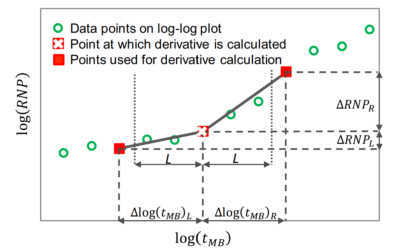
Fig. 2: Bourdet derivative
It is different from a weighted central difference in the way that it uses a constant log-cycle window size, L, on both sides of the point of derivation. A weighted central difference, on the other hand, uses a constant index step size, e.g. i-5 and i+5 for step size of 5, on each side of the point of derivation. The window size, L, represents the log-cycle fraction used to control the amount of smoothing. Typical values are 0.01 to 0.2. The default L in whitson+ is 0.2. The larger the L value, the more smoothing.
The Bourdet algorithm implemented in whitson+ was provided by Behnam Zanganeh.
1.7.3. Weighted Central Difference
The weighted central difference is given by,
where the \(L\)-subscript refers to the index to the left with a constant step size, \(S\), i.e. \(i-S\) and the \(R\)-subscript refers to the index to the right with a constant step size, \(S\), i.e. \(i+S\).
1.7.4. Central Difference
This is the naive implementation, given by three points per derivative for central difference in the following manner
1.7.5. Derivatives in Material Balance Time
Because of noise in real field data, material balance time may not be in sequence. This might cause problems in derivative calculations. Hence, the data must be sorted in terms of increasing material balance time prior to calculating the derivative. The following procedure, adapted from Samandarli et al.(2012), is used for this purpose.
- RNP and material balance time \((t_c)\) are calculated at each real time step.
- RNP and \((t_c)\) are sorted in increasing order of material balance time, with repeat material balance times eliminated.
- The RNP derivative, RNP', is then calculated using the sorted data.
1.8. RTA Integrals
In the case of complex and noisy data, Blasingame et al. [1] introduced the concepts of pressure-integral and pressure-integral difference, which have become essential tools for the scrutiny of well-test data through type-curve analysis. Similarly, McCray (1990) presented the idea of the rate-integral and rate-integral derivative, which was utilized by Blasingame and his students and colleagues for type-curve analysis of production data in various publications.
1.8.1. The Rate Normalized Pressure (RNP) Integral
The use of the RNP integral and its derivative was suggested by Chu et al. [6] for the study of flow-regime signature in the Wolfcamp shale. For liquids, the equations are written as follows:
The integral can be calculated using various time functions (real time or linear superposition time); here it is presented in material balance time for illustration.
As with and , the calculations for and can be applied to gases through inclusion of gas pseudovariables.
1.8.2. Discrete Calculation
The discrete form of Eq. \eqref{eq:RTA-integral} is expressed in the following manner:
1.8.3. LFP (A√k) Adjustments
The conversion from a slope to LFP (A√k) while using the RNP integral must be adjusted by 2/3 to ensure that the LFP is calculated correctly from the slope. This follows from integrating the RNP as a function of √t.
When turning on the integral function, this correction is applied
1.9 Flow Regimes
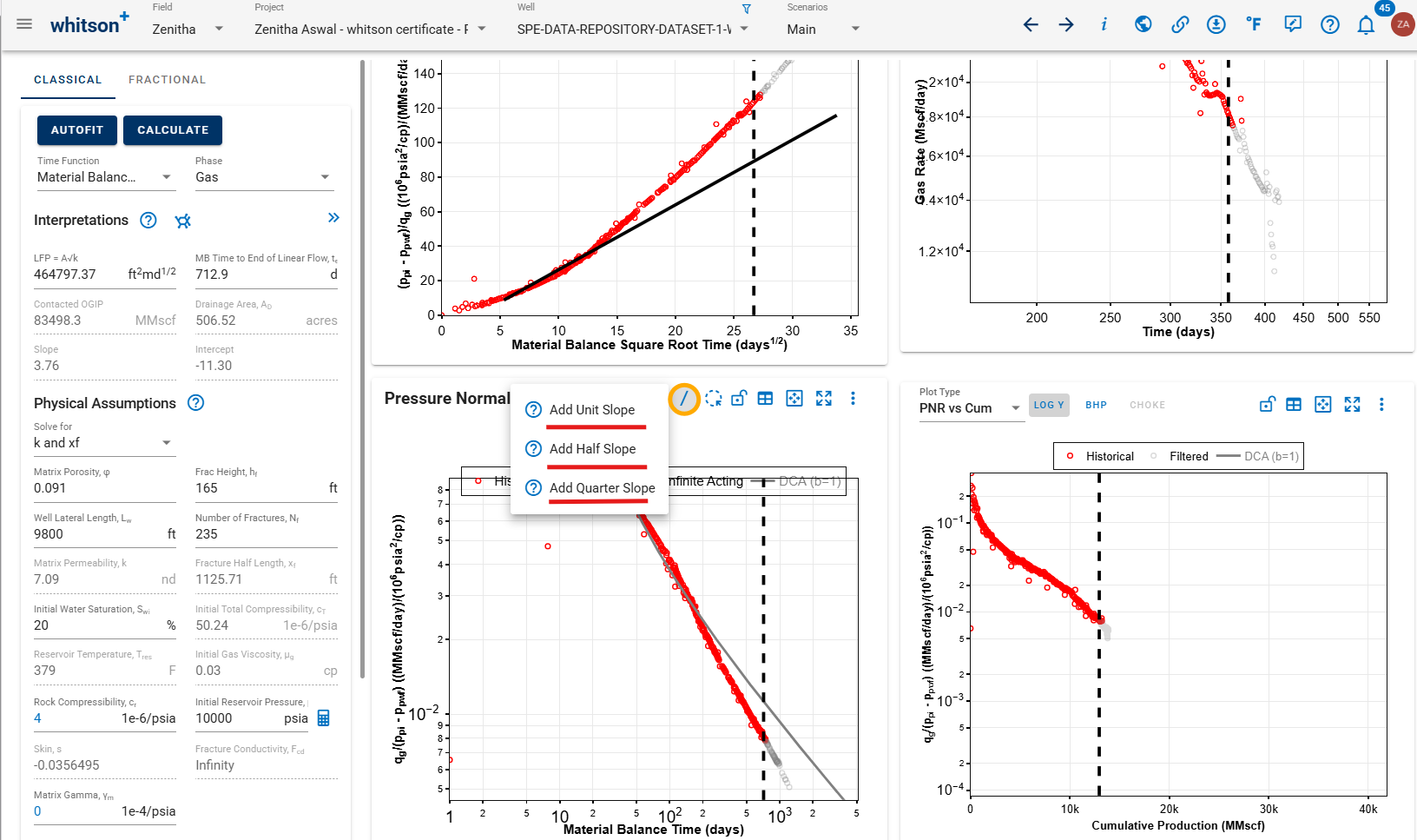
The Pressure Normalized Rate (PNR) plot (log-log plot of PNR vs t) can be used as a diagnostic plot to identify the flow regimes in different portions of the well data (early, middle and late time). The flow regimes represent the way the fluid flows into the wellbore, often a function of shape and size of the reservoir, well completion, and duration of flow. Each flow regime is identified by the data showing a characteristic slope on this log-log plot.
whitson+ offers the ability to add 3 different interpretation lines using the '/' button on the PNR plot. These lines are aligned with the data for interpreting the flow regime and can be broadly associated with the following:
| Interpretation Line | Slope Value | Flow Regime |
|---|---|---|
| Quarter Slope | -1/4 | Bilinear Flow (low Fcd wells) |
| Half Slope | -1/2 | Infinite-Acting Linear Flow (typical in MFHW) |
| Unit Slope | -1 | Pseudo-steady-State / Boundary-Dominated Flow |
Interpretation of flow regimes can be highly subjective since these flow regimes do not have sharp transitions and may present long transient periods between them - especially in low permeability, unconventional reservoirs and multi-fractured horizontal wells (MFHW). It is also important to be aware of the time scale and order of the interpretation when identifying flow regimes. For example, a unit slope at early time could mean wellbore storage while a unit slope at late time is more likely to mean pseudo-steady state flow or boundary dominated flow. Bilinear flow (quarter slope) is typically observed at very early time prior to the onset of linear flow (half slope). The identification and analysis of these flow regimes are crucial for optimizing reservoir management strategies.
You can also aid the interpretation by plotting the data derivative, switching between various time functions available, and using the lasso filter tool on the RNP plot (above the PNR plot) to highlight different sections of the data.
1.10. Solutions of Linear Flow - Surface Oil Rates
Combining constant rate (variable pressure) solution with superposition time allows to account for variable rate solution.
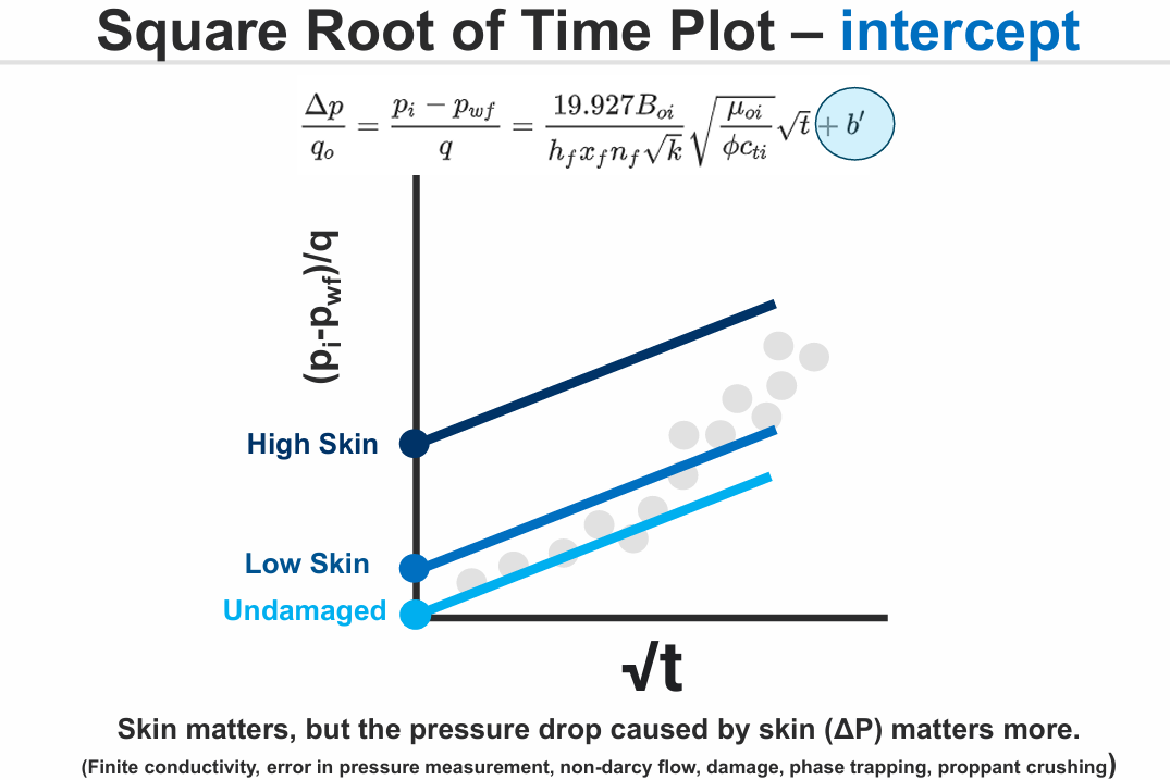
Theoretically, linear flow can be defined in terms of square root of time as follows:
| Phase | Linear Flow Equation at Constant Rate |
|---|---|
| Oil | \begin{equation} \label{eq:CR-linear-oil} \frac{\Delta p}{q_o} = \frac{p_i-p_{wf}}{q_o} = \frac{19.927B_{oi}}{h_fx_fn_f\sqrt{k}} \sqrt{\frac{\mu_{oi}}{\phi c_{ti}}} \sqrt{t}+b' \end{equation} |
| Gas | \begin{equation} \label{eq:CR-linear-gas} \frac{\Delta p_{pg}}{q_g} = \frac{p_{p_i}-p_{p_{wf}}}{q_g} = \frac{200.8T_R}{h_fx_fn_f\sqrt{k}} \frac{1}{\sqrt{(\phi\mu_gc_t)_i}} \sqrt{t}+b' \end{equation} |
| Water | \begin{equation} \label{eq:CR-linear-water} \frac{\Delta p}{q_w} = \frac{p_i-p_{wf}}{q_w} = \frac{19.927B_{wi}}{h_fx_fn_f\sqrt{k}} \sqrt{\frac{\mu_{wi}}{\phi c_{ti}}} \sqrt{t}+b' \end{equation} |
| Hydrocarbon | \begin{equation} \label{eq:CR-linear-hc} \frac{\Delta p}{q_{hc}} = \frac{p_i-p_{wf}}{q_{hc}} = \frac{19.927}{h_fx_fn_f\sqrt{k}} \sqrt{\frac{\mu_i}{\phi c_{ti}}} \sqrt{t}+b' \end{equation} |
| Liquid | \begin{equation} \label{eq:CR-linear-liq} \frac{\Delta p}{q_{liq}} = \frac{p_i-p_{wf}}{q_{liq}} = \frac{19.927}{h_fx_fn_f\sqrt{k}} \sqrt{\frac{\mu_i}{\phi c_{ti}}} \sqrt{t}+b' \end{equation} |
| Total | \begin{equation} \label{eq:CR-linear-total} \frac{\Delta p}{q_{tot}} = \frac{p_i-p_{wf}}{q_{tot}} = \frac{19.927}{h_fx_fn_f\sqrt{k}} \sqrt{\frac{\mu_i}{\phi c_{ti}}} \sqrt{t}+b' \end{equation} |
| Oil Pseudopressure | \begin{equation} \label{eq:oilpp} \frac{\Delta p_{po}}{q_o} = \frac{p_{p_i}-p_{p_{wf}}}{q_o} = \frac{19.927B_{oi}}{h_fx_fn_f\sqrt{k_i}} \sqrt{\frac{\mu_{oi}}{\phi c_{ti}}} \sqrt{t}+b' \end{equation} |
Pseudo Viscosity Calculations
For liquid rates, a "pseudo" liquid viscosity is calculated as the saturation weighted average viscosity, as follows
For total rates, a "pseudo" total viscosity is calculated as the saturation weighted average viscosity, as follows
in which \(B_o\) is oil formation volume factor in RB/STB, \(B_w\) is water formation volume factor in RB/STB, \(T_R\) is reservoir temperature in rankine, \(\phi\) is porosity in fraction, \(\mu\) is viscosity in cp, \(c_t\) is total compressibility in 1/psi and \(k\) is permeability in md. Fracture height and half-length in feet are denoted by \(h\) and \(x_f\), respectively. Number of fracture is denoted by \(n_f\). Initial and flowing bottomhole pressure are \(p_i\) and \(p_{wf}\) in psia. Water viscosity, \(\mu_w\), is set to 0.5 cp.
Total compressibility accounts for the compressibility of the fluid phases present in the system as well as the rock compressibility and is written as
where \(c_g\), \(c_o\), \(c_w\) and \(c_r\) denote gas, oil, water and formation (rock) compressibility, respectively. The default value of \(c_r\) is 4x10\(^{-6}\) 1/psi and \(c_w\) is 2.8x10\(^{-6}\) 1/psi in whitson+.
\(\Delta p_p\) is real gas pseudo-pressure drop defined as
What is pseudopressure, why we need it, and how to calculate it?
The governing equation for fluid flow in a reservoir is similar for both liquids and gases. However, solving the gas flow equation directly is challenging due to the nonlinear behavior of gas properties—particularly compressibility and viscosity—as functions of pressure.
To simplify the mathematics, two key assumptions are typically made in the derivation of the flow equation:
-
Constant compressibility
-
Constant viscosity
These assumptions are often valid for liquids, where both viscosity and compressibility vary little with pressure, enabling the governing equation to become linear.
For gases, however, these assumptions break down except at high pressures. Gas compressibility and viscosity are highly pressure-dependent, and ignoring their variation can lead to significant errors in production and pressure data analysis.
To address this, Al-Hussainy and Ramey (1970s) introduced a rigorous approach using the concept of gas pseudopressure. This transformation linearizes the gas flow equation by incorporating the pressure dependence of gas viscosity and compressibility. The pseudopressure at reservoir pressure and at flowing bottomhole pressure is defined as follows:
What is pseudotime, Why is it needed, and How is it calculated?
What is pseudotime: For gas reservoir, using pseudopressure is often not enough to fully linearize the diffusivity equation. While pseudopressure accounts for the pressure dependence of gas viscosity and gas compressibility factor, the accumulation term in the gas diffusivity equation still contains gas compressibility and viscosity, which also vary with pressure. As a result, real time is not always the most appropriate time variable for gas-well analysis. Why is it needed: To address this, the concept of pseudotime was introduced. Gas pseudotime is a transformed time variable that accounts for pressure-dependent changes in gas viscosity and total compressibility in the gas diffusivity equation. By replacing real time with pseudotime, the effect of varying gas properties during drawdown is incorporated into the pseudotime term. When used together, pseudopressure and pseudotime allow the gas-flow equation to be written in a form analogous to that of a slightly compressible liquid. This provides the basis for applying many liquid-flow solutions to gas systems.
Mathematically, pseudotime is defined as:
where \((\mu_{g}c_t)\) is evaluated at initial conditions, and \(\mu_g (p_{ref})\) and \(c_t (p_{ref})\) are evaluated at a selected reference pressure. Unlike pseudopressure, which is obtained from an exact pressure integral, pseudotime is evaluated through time integration and therefore requires a representative pressure to be specified for calculating pressure-dependent gas properties over each integration interval.
The selection of the reference pressure depends on the type of reservoir and the analysis being performed. In production data analysis for conventional gas reservoirs, including methods such as Type Curve Analysis and Flowing Material Balance, the reference pressure used to evaluate gas properties is commonly taken as the average reservoir pressure, \(\bar p\). In many conventional gas reservoirs, boundary-dominated flow is reached relatively early in the producing life of the well. As a result, average reservoir pressure often provides a reasonable and practical reference pressure for calculating pseudotime.
However, in the analysis of production data from multifractured horizontal wells (MFHWs) in low-permeability reservoirs, transient flow commonly persists for a substantial portion of the production history. Under these conditions, average reservoir pressure may not adequately represent the pressure behavior of the actively contributing region. As suggested by Anderson and Mattar (2007), gas properties are instead evaluated using the average pressure within the region of investigation, \(\bar p_{inv}\). When this reference pressure is used, the resulting time function is commonly referred to as corrected pseudotime, \((t_{ca})\).
How is it Calculated: Corrected pseudotime is calculated by first determining the average pressure within the region of investigation, \(\bar p_{inv}\), as a function of time. This pressure is obtained by applying the gas material-balance equation to the contacted gas volume:
where \(G_p (t)\) is cumulative gas production:
and \(G_{inv} (t)\) is the contacted gas-in-place. The contacted gas-in-place is calculated from the gas volumetric relationship:
where \(A_{inv} (t)\) is the area of the region of investigation, \(h\) is the net pay thickness, \(\phi\) is porosity, \(S_{gi}\)is initial gas saturation, and \(B_{gi}\) is the initial gas formation volume factor. The area \(A_{inv} (t)\) depends on the reservoir geometry and the distance of investigation, \(y_{inv}\). For linear flow geometry,
The distance of investigation during linear flow is given by:
which shows that the contacted region grows with the square root of time.
By substituting Eqs. (8) through (11) into the material-balance expression (Eq. 7) and simplifying, the following relationship is obtained
where LFP is given by:
To evaluate \(\bar p_{inv}\) from Eq. (10), the LFP must first be determined. As discussed in the Linear Flow Parameter section, LFP is obtained from \(m_{CR}\), the slope of the straight line fitted to rate-normalized pseudopressure, \(\ \frac {p_{pi}- p_{pwf}}{q_g}\), plotted versus the square root of linear superposition corrected pseudotime, \(\sqrt {t_{ca}}\). Because corrected pseudotime depends on the average pressure within the region of investigation used to evaluate gas properties, while that pressure is itself determined from LFP, the calculation is inherently iterative.
The following GIF illustrates how adjusting the slope of the line also changes the calculation of the linear-superposition corrected pseudotime.
In specialized plot, the vertical dashed line indicates the time to the end of linear flow, \(t_{elf}\), where the flow regime transitions from transient flow to boundary-dominated flow. At this point, the well drainage area is considered fully contributing to flow, and the region of investigation is no longer increasing with time. Consequently, the average reservoir pressure calculation is revised to use a fixed OGIP at \(t_{elf}\). The choice of \(t_{elf}\) affects only the production data after the end of linear flow and has no impact on the data before \(t_{elf}\). For times after \(t_{elf}\), the material balance equation is modified accordingly.
The GIF below demonstrates how the location of the vertical line affects the data calculation.
According to Eqs. \eqref{eq:CR-linear-oil}, \eqref{eq:CR-linear-gas}, \eqref{eq:CR-linear-water} the plot of rate normalized pressure \(\left(\frac{\Delta p}{q}\right)\) vs. square root of time \(\sqrt{t}\) (or square root of material balance time \(\sqrt{t_c})\) generates a straight line. The slope of this line is given by
| Phase | Equation of Slope |
|---|---|
| Oil | \begin{equation} \label{eq:CR-m-oil} m_{CR} = \frac{19.927B_o}{h_fx_fn_f\sqrt{k}} \sqrt{\frac{\mu_o}{\phi c_t}} \end{equation} |
| Gas | \begin{equation} \label{eq:CR-m-gas} m_{CR} = \frac{200.8T_R}{h_fx_fn_f\sqrt{k}} \frac{1}{\sqrt{(\phi\mu_gc_t)_i}} \end{equation} |
| Water | \begin{equation} \label{eq:CR-m-water} m_{CR} = \frac{19.927B_w}{h_fx_fn_f\sqrt{k}} \sqrt{\frac{\mu_w}{\phi c_t}} \end{equation} |
| Hydrocarbon, Liquid, and Total | \begin{equation} \label{eq:CR-m-total} m_{CR} = \frac{19.927}{h_fx_fn_f\sqrt{k}} \sqrt{\frac{\mu}{\phi c_t}} \end{equation} |
| Oil Pseudopressure | \begin{equation} \label{eq:CR-m-oil-pseudo} m_{CR} = \frac{19.927B_{oi}}{h_fx_fn_f\sqrt{k_i}} \end{equation} |
Subscript \(CR\) is to emphasize the variable of constant rate solution.
1.11. Skin and Fracture Conductivity
The intercept (\(b'\)) from the linear flow equation is a result of near well effects, e.g. skin \((s')\) and finite fracture conductivity \((F'_{cd})\). The unit of the intercept is psi/STB/d.
Skin is defined as follows:
| Phase | Equation of Skin |
|---|---|
| Oil | \begin{equation} \label{eq:s-oil} s'= \frac{b'k\left(2x_fn_f\right)} {141.2B_o\mu_o} \end{equation} |
| Gas | \begin{equation} \label{eq:s-gas} s'= \frac{b'k\left(2x_fn_f\right)} {1.417\times10^6T_R} \end{equation} |
| Water | \begin{equation} \label{eq:s-water} s'= \frac{b'k\left(2x_fn_f\right)} {141.2B_w\mu_w} \end{equation} |
| Hydrocarbon, Liquid, and Total | \begin{equation} \label{eq:s-total} s'= \frac{b'k\left(2x_fn_f\right)} {141.2\mu} \end{equation} |
Where \(n_f\) represents effective fractures number.
Fracture conductivity is defined as follows:
| Phase | Equation of Fracture Conductivity |
|---|---|
| Oil | \begin{equation} \label{eq:Fcd-oil} F'_{cd} = \frac{141.2B_o\mu_o} {b'khn_f} \left( 1+\frac{h}{x_f} \left[ \ln\left(\frac{h}{2r_w}\right) -\frac{\pi}{2} \right] \right) \end{equation} |
| Gas | \begin{equation} \label{eq:Fcd-gas} F'_{cd} = \frac{1.417\times10^6T_R} {b'khn_f} \left( 1+\frac{h}{x_f} \left[ \ln\left(\frac{h}{2r_w}\right) -\frac{\pi}{2} \right] \right) \end{equation} |
| Water | \begin{equation} \label{eq:Fcd-water} F'_{cd} = \frac{141.2B_w\mu_w} {b'khn_f} \left( 1+\frac{h}{x_f} \left[ \ln\left(\frac{h}{2r_w}\right) -\frac{\pi}{2} \right] \right) \end{equation} |
| Hydrocarbon, Liquid, and Total | \begin{equation} \label{eq:Fcd-total} F'_{cd} = \frac{141.2\mu} {b'khn_f} \left( 1+\frac{h}{x_f} \left[ \ln\left(\frac{h}{2r_w}\right) -\frac{\pi}{2} \right] \right) \end{equation} |
Where \(r_w\) (equal 1 ft) indicates well radius in ft and \(n_f\) represents effective fractures number.
1.12. Linear Flow Parameter
The linear flow parameter (LFP) is expressed in terms of slope of the straight line as:
| Phase | Equation of Linear Flow Parameter |
|---|---|
| Oil | \begin{equation} LFP=A\sqrt{k} = 4\cdot \frac{19.927B_o}{m_{CR}} \sqrt{\frac{\mu_{oi}}{\phi c_{ti}}} \end{equation} |
| Gas | \begin{equation} LFP=A\sqrt{k} = 4\cdot \frac{200.8T_R}{m_{CR}} \sqrt{\frac{1}{(\phi\mu c_t)_i}} \end{equation} |
| Water | \begin{equation} LFP=A\sqrt{k} = 4\cdot \frac{19.927B_w}{m_{CR}} \sqrt{\frac{\mu_{wi}}{\phi c_{ti}}} \end{equation} |
| Hydrocarbon, Liquid, and Total | \begin{equation} LFP=A\sqrt{k} = 4\cdot \frac{19.927}{m_{CR}} \sqrt{\frac{\mu_i}{\phi c_{ti}}} \end{equation} |
1.13. Distance of Investigation
It is important to be able to establish the end of the linear flow where the slope on the square root of time plot start to depart from being a straight line. The time to end of linear flow \((t_{elf})\) is key to specify the drainage volume, and to resolve estimates of parameters such as \(k\) and \(x_f\).
Generally, distance of investigation \((y_e)\) can be determined by dividing well horizontal length \((L_w)\) with effective fractures number \((n_f)\).
The constant rate solution of \(y_e\), or the distance to the outer boundary is described as
Combining Eqs. \eqref{eq:ye-Lw} and \eqref{eq:CR-ye} gives
The time to end of linear flow \((t_{elf})\) can be solved by rearranging Eq. \eqref{eq:CR-ye-2}
In the case of no deviation of production data from straight line, the latest production time should be used as \(t_{elf}\) which will generate the minimum drainage volume.
1.14. Permeability and Fracture Half-length
1.14.1. Permeability
Rearranging Eq. \eqref{eq:CR-ye-2} to get permeability will result in
1.14.2. Fracture half-length
LFP can also be defined as
in which \(A\) is total effective fracture surface area in ft\(^2\) defined as
After determining LFP and \(k\) previously, \(x_f\) can be calculated straightforward by rearranging Eqs. \eqref{eq:LFP} and \eqref{eq:total-area-to-flow}.
1.15. Contacted Pore Volume, Drainage Area and Hydrocarbons-in-place
Having all the necessary variables, the contacted pore volume in ft\(^3\) can be easily determined by:
Drainage area \(A_d\) in acres (1 acre = 43,560 ft\(^2\)) is defined as
An alternative way to calculate drainage \(A_d\) is
In which 7758 is a conversion factor from acre-ft to bbl.
Original hydrocarbons-in-place are calculated using the following relationships:
For oil:
For gas:
For water:
1.16. Production Forecast
With simple decline curve analysis, the production forecast can be projected. The classic arps hyperbolic decline is written as
Flow production rate and nominal decline rate at the start of forecast are depicted by \(q_i\) and \(a_i\), respectively. Flow production rate at time \(t\) is \(q(t)\) while \(b\) is rate exponent. In this module, the production forecast is start at the end of the linear flow \((t_{elf})\), thus the other variables are with respect to \(t_{elf}\).
Production forecast rate is calculated by rewriting Eq. \eqref{eq:arps-dca}
A more detailed explanation of decline curve analysis can be found here.
1.17. Geomechanical Effects - Pressure-Dependent Permeability
For gas reservoirs, the matrix can be assigned a pressure-dependent permeability on the form
where \(k_m(p)\) is a dimensionless permeability multiplier.
and \(\gamma_r\) is a property that be assigned in the frontend. To activate the pressure-dependent permeability, make \(\gamma_r\) a non-zero value.
To incorporate a variation of permeability with pressure into the pseudo-pressure term, the definition of pseudo-pressure is modified as follows
To incorporate a variation of permeability with pressure into the pseudotime term, the definition of corrected pseudotime is modified as follows:
Geomechanical effects can also be added in both the matrix and fracture in the numerical model.
For a given dataset, a higher gamma value—reflecting productivity loss due to pressure-dependent permeability—requires more / to achieve the same and production rate.
1.18. Computing Original Gas in Place with Adsorption
Shale reservoirs possess a remarkable capacity to store methane through a process known as "adsorption." This involves gas molecules adhering to the organic material within the shale, creating a near-liquid state of condensed gas. A useful analogy is to envision a magnet sticking to a metal surface or lint clinging to a sweater, illustrating the concept of adsorption versus absorption, where one substance is trapped inside another like a sponge soaking up water. The adsorption process is reversible due to its reliance on weak attraction forces.
Compared to conventional reservoirs, shale reservoirs can store significantly more gas in the adsorbed state, even when compression is applied at pressures below 1000 psia. Notably, the gas stored in shale is predominantly held in the adsorbed state, as opposed to being free gas. This is because the volume of the cleat or fracture system within shale is relatively small compared to the overall reservoir volume. As a result, the pressure volume relationship is commonly described through the desorption isotherm alone.
Langmuir Isotherm
The release of adsorbed gas is commonly described by a pressure relationship called the Langmuir isotherm. The Langmuir adsorption isotherm assumes that the gas attaches to the surface of the shale, and covers the surface as a single layer of gas (a monolayer). At low pressures, this dense state allows greater volumes to be stored by sorption than is possible by compression.
The typical formulation of the Langmuir isotherm is:
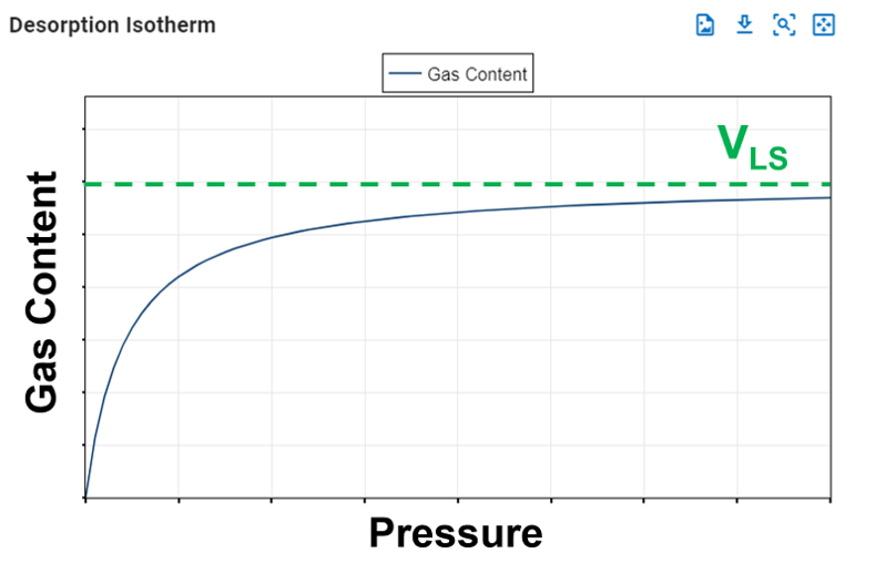
Langmuir Volume, VLS
The Langmuir volume is the maximum amount of gas that can be adsorbed by a shale at an "infinite pressure". The plot below of a Langmuir isotherm demonstrates that gas content asymptotically approaches the Langmuir volume as pressure increases to infinity.
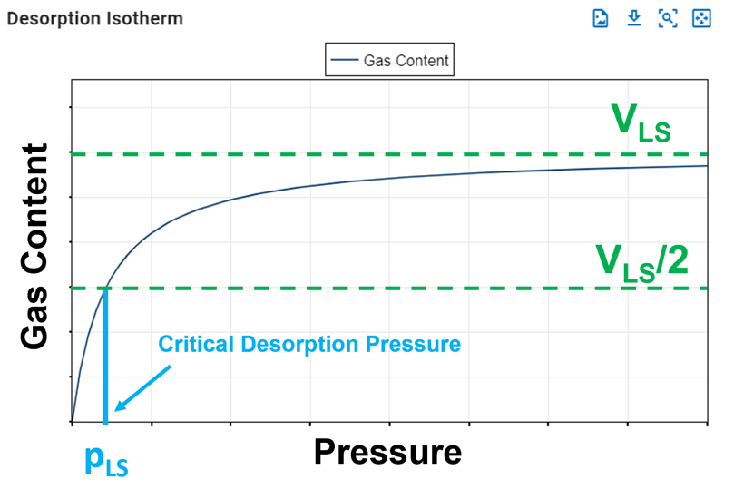
Langmuir Pressure, pLS
The Langmuir pressure, or critical desorption pressure, is the pressure at which one half of the Langmuir volume can be adsorbed. As seen in the figure below, it changes the curvature of the line and thus affects the shape of the isotherm.
Computing Original Gas in Place (OGIP)
Ambrose et al.[1] argue that the free OGIP must be corrected for the adsorbed gas that occupies some of the hydrocarbon pore volume (HCPV). If porosity is estimated from core plugs where core preparation has removed the adsorbed gas, then the OGIP will be overestimated.
The convention of reporting OGIP when adsorption is included, is to report it in units of scf/ton (standard cubic feet per short ton). For a fluid system having only dry/wet gas and water, the total OGIP is
where
and with \(C_1\approx 5.7060\) and \(C_2\approx1.318\cdot10^{-6}\) are unit conversion factors. The shale saturation is capped at \(1-S_{wi}\), meaning the maximum amount of shale you can have is the entire HCPV. Hence, this will make the results independent of the adsorption numbers when violating this constraint.
The OGIP resolved in the ARTA and GFMB features yields the free OGIP. We can use this volume to compute the rock mass, which in turn can be used to calculate the adsorbed OGIP. Multiplying equation \eqref{eq:freegasperton} with the rock mass (\(G=\hat{G}_f m_r\)) gives the free OGIP in units of scf. Solving for the rock mass yields
This rock mass can then be multiplied by equation \eqref{eq:adsorbedgasperton} to get the adsorbed OGIP in scf, i.e.,
Total Compressibility when Adsorption is ON
In order to honor mass balance, it becomes necessary to modify total system compressibility when accounting for adsorption. Total system compressibility can be determined using the following equation:
The derivation of this equation is shown here and is constructed upon Ambrose et al.[1].
1.19. Estimate Initial Reservoir Pressure from Square Root Time Plot

To estimate the initial reservoir pressure () from the plot, the algorithm automatically varies () in increments rounded to the nearest 100 psia (or 700 kPaa / 7 bara) to find the best linear fit through the origin. The pressure range explored spans from -2000 psia below to +10000 psia above the maximum bottomhole pressure observed during the first 100 days of hydrocarbon flow. The first 5 days are ignored as they are typically associated with data quality issues. Upon completion, the optimum initial reservoir pressure, the best-fit slope and and corresponding early-time linear flow time () are assigned to the well.
1.20. Calculation of (Coefficient of Determination)
In whitson+, is used to evaluate the quality of a linear regression fit. It measures how well the regression line explains the variability of the observed data. Its value ranges from zero to one, where values closer to one indicate a stronger linear fit.
- equation for regression through the origin
- equation for regression with an intercept
1.21. Limitations of Classical RTA
One of the key limitations of classical RTA is the single-phase flow assumption. This is a good assumption for dry and wet gas reservoirs, and when producing with flowing pressures above the saturation pressure. However, for wells producing below the saturation pressure, the single-phase flow assumption is not valid. Hence, using the classical RTA equations for wells subject to multiphase flow effects might skew the interpretation. If the saturation pressure coincides with the change of slope on the square root of time plot, as seen in Fig.2, the slope change might just be an artifact of multiphase flow. To account for the multiphase flow effects, we recommend using the numerical RTA workflow. More info can be found here.
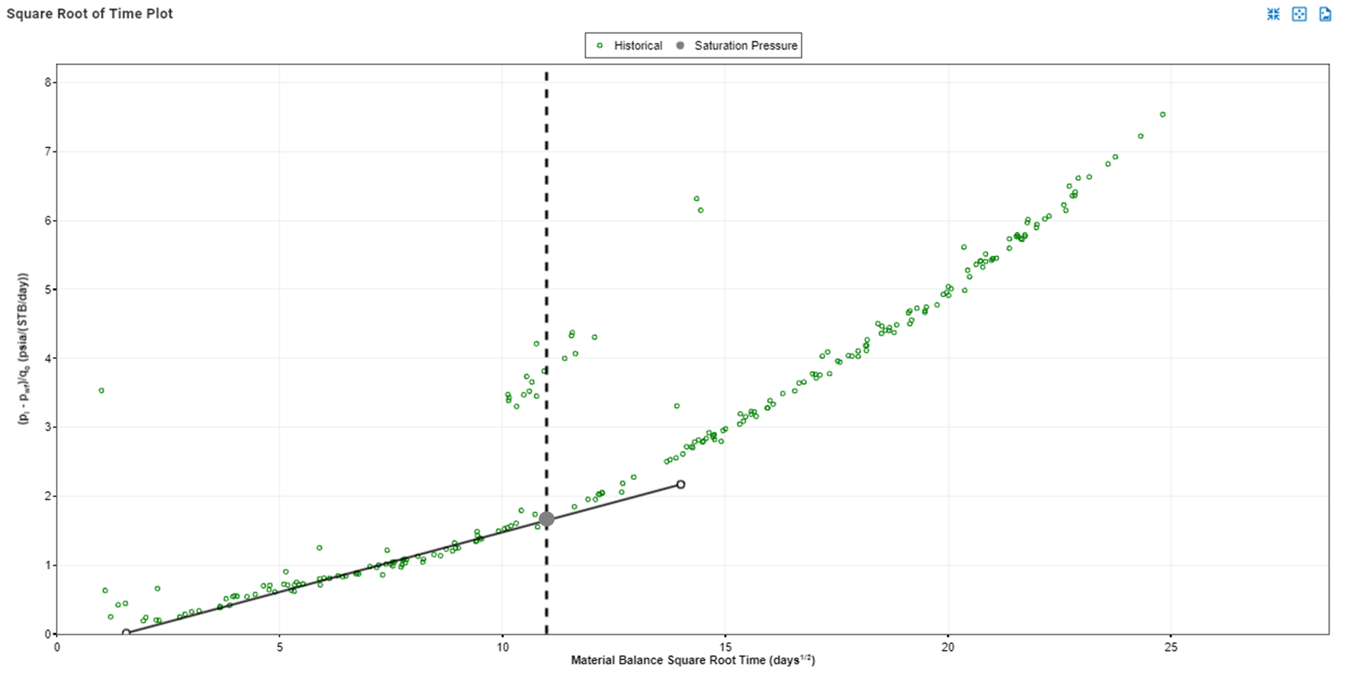
Fig. 2: Slope change coinciding with well dropping below the saturation pressure might be an artifact of multiphase flow.
2. Empirical Assumptions - EUR
This feature uses empirical assumptions after the time to end of linear flow () by simply fitting an Arps equation through the historical data.
The EUR option is available for all time functions, however, forecasting should be performed in real time to ensure accuracy. This approach avoids inconsistencies, such as differences in -factor handling between real-time and material balance time. For example, the -factor for BDF is set to 1 (harmonic) in material balance time, while it is 0 (exponential) in real time.
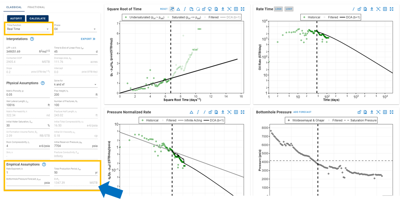
Key DCA inputs - \(b\)-factor to use for the PNR vs time plot, pwf - the abandonment pressure to dictate your BHP or drawdown in the future, other settings for forecast period, limiting decline segment, cut off rates etc.
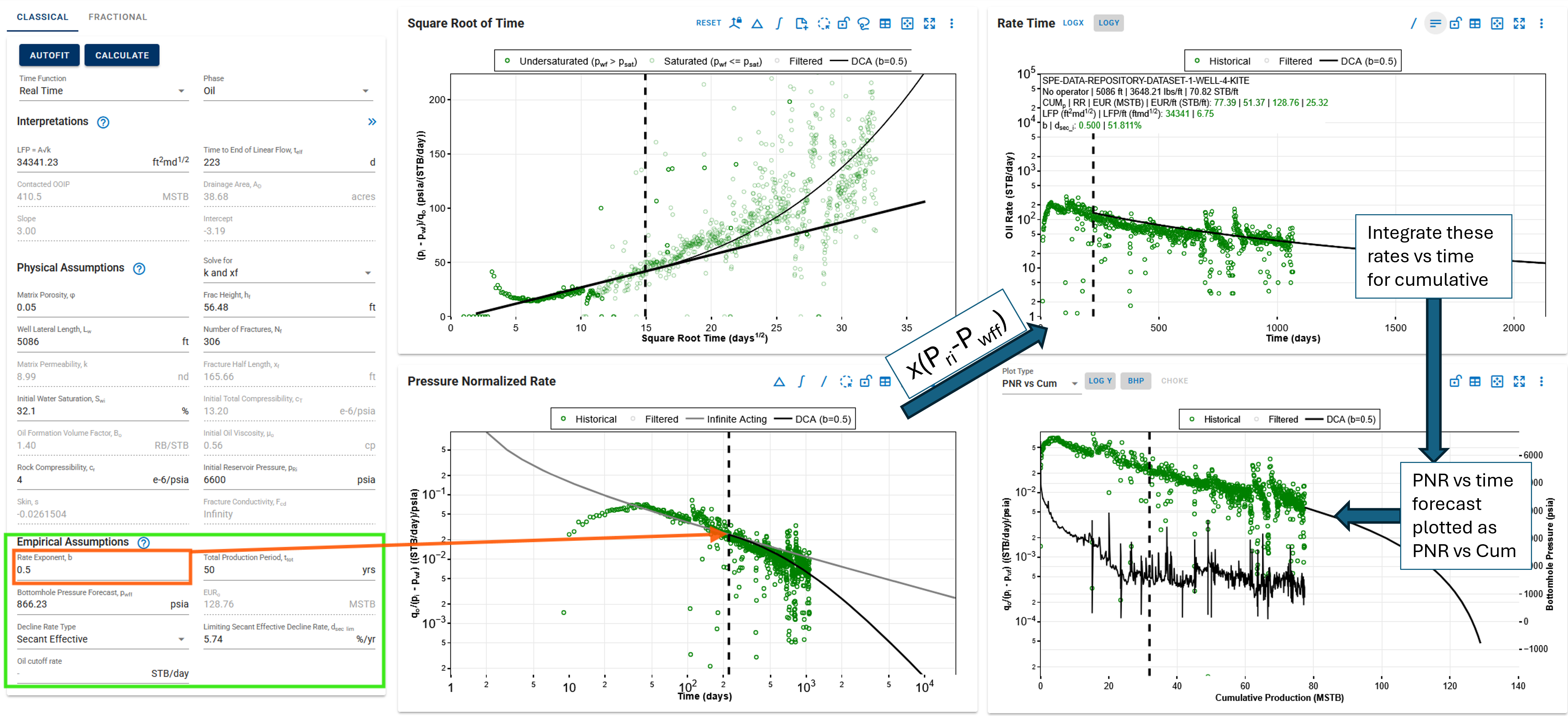
2.1. Analytical RTA DCA - Plot PNR vs Cumulative forecast
The DCA part of the analytical RTA is simply a way to forecast the PNR vs time plot with DCA, then use the abandonment pressure to calculate the rate equivalent of a constant pressure drawdown (i.e. initial pressure - abandonment pressure, for the entire forecast) for this PNR decline. We then calculate the cumulative of these forecasted rates vs time to plot the PNR vs Cum forecast.
In summary, PNR vs Cum forecast is calculated in 3 steps (arrows):
Interpreting PNR Forecast vs. Time Plots
The PNR vs Time plot, the forecast is always plotted as a deviation from the Infinite Acting line (from your LFP pick), at the time to end of linear flow. The other plots may show a disconnect in the historical and forecast rate data if the abandonment pressure is not the same as the BHP on the last producing day.
This is how the EUR is calculated using DCA in Analytical RTA.
3. Comments on Use of Material Balance Time
-
If the analytical solutions are plotted to fully-penetrating fracture problem for either a constant rate or constant pressure case (Eqs. 2 and 3 in Wattenbarger et al. (1998)), a half-slope on a log-log plot should be expected during infinite acting (IA) period with a constant difference between the two solutions of a factor \(\frac{\pi}{2}\). The constant pressure solution in the boundary-dominated flow (BDF) period will exhibit an exponential function, whereas the constant rate solution in the BDF will exhibit a unit-slope.
-
If one plots the constant pressure solution versus material balance time, then the curve will (1) overlap the constant rate solution in the BDF period (because material balance time applies rigorously in the BDF period) and, (2) approximate the constant rate solution in the IA period (i.e. it plots close to the true solution, but not on top of it as in the BDF period).
-
Because the material balance time solution is only an approximate solution in the IA period, the resulting key numbers (e.g. \(x_f\) and \(k\)) will not be the exact numbers you expect, at least for simple synthetic cases (e.g. a low GOR oil with constant \(p_{wf}\)). However, for a variable rate and pressure solution (real life), one can only get the true values by rigorous superposition (or de-superposition), and thus an approximate solution by the use of material balance time is likely good enough.
4. Which phase or time function should I pick?
First, consistency is paramount. When comparing different wells using analytical RTA, ensure all evaluations are conducted using the same phase (primary, liquid, total or hydrocarbon).
Second, double-check that your selected slope and LFP values align with the half-slope on the PNR plot (see below).
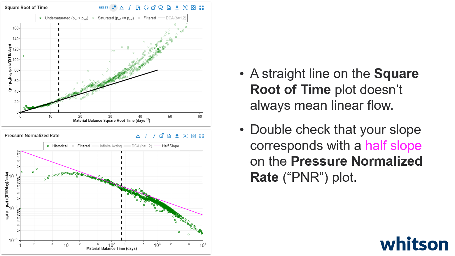
Analytical RTA does not rigorously account for the combined effects of superposition and multiphase flow. Therefore, it is not recommended to use analytical RTA to determine contacted pore volume or any other reservoir property. This method doesn’t account for the combination of superposition and PVT/multiphase flow effects.
4.1. Why do we still use Analytical RTA?
- Familiarity: It is readily available within industry-standard software and many practitioners are accustomed to using it.
- Suitability for single-phase areas: e.g. dry gas basins.
- Rapid LFP estimation: ARTA can be effectively used to quickly estimate single-phase LFP values for a large number of wells. While the accuracy may be limited, the consistent application of assumptions ensures comparable results across the dataset.
The choice of time function for linear flow analysis is a matter of preference and subject to ongoing debate.
Strictly speaking, the specialized plot for linear flow utilizes the square root of real time to calculate LFP and the time to the end of linear flow. However, the LFP equation itself only specifies 'time' and does not explicitly define which time function should be used. Consequently, when material balance time is employed, you can still derive LFP and OOIP by determining the time to the end of linear flow. However, the calculated values for LFP and OOIP will differ from those obtained using real time.
4.2. Practical Considerations and Limitations of Analytical RTA
In practice, we have observed operators utilizing both real time and material balance time for linear flow analysis. It is crucial to acknowledge the inherent limitations of Analytical RTA, such as its reliance on single-phase assumptions, low fluid compressibility assumptions, and the use of initial PVT properties like viscosity. Therefore, the absolute values of LFP and OOIP derived from Analytical RTA should be interpreted with caution. Instead, these values are more valuable for qualitative comparisons between wells, rather than for precise quantitative estimations.
In summary, consistently use a single time function as the basis for your analysis to ensure comparability of LFP values across wells.
Furthermore, consider the following guidelines for time function selection based on your analytical objectives:
-
For tying to DCA, use real time.
-
If you aim to resolve reservoir parameters using the constant rate analytical solution, employ material balance time.
-
If your primary goal is to quantify LFP, linear superposition time can be used.
5. LFP Differences between Analytical, Fractional and Numerical RTA
Numerical RTA generally yields a greater LFP value compared to Analytical RTA.
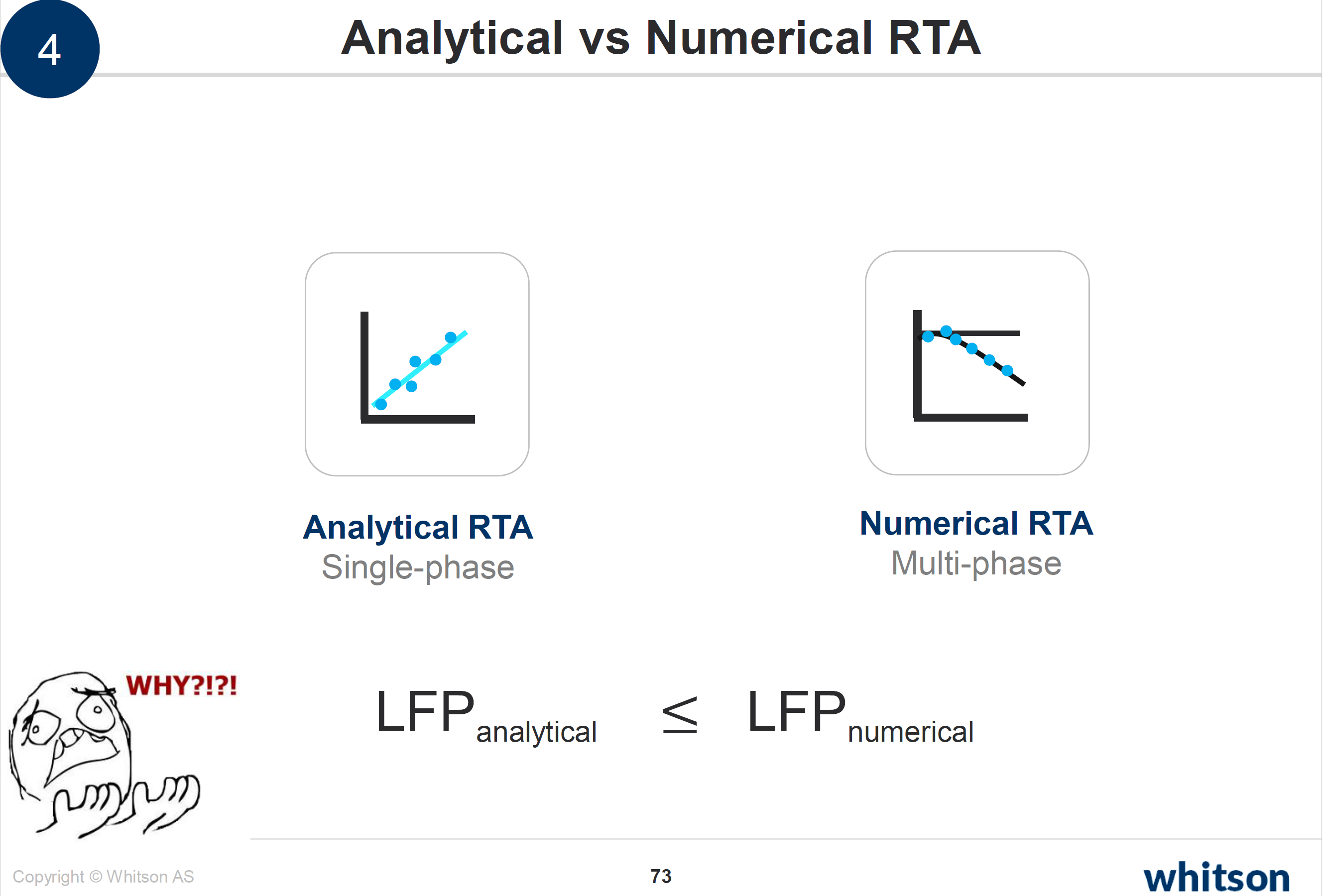
Given that each technique calculates LFP slightly differently, comparisons of LFP values should be made between wells using the same technique.
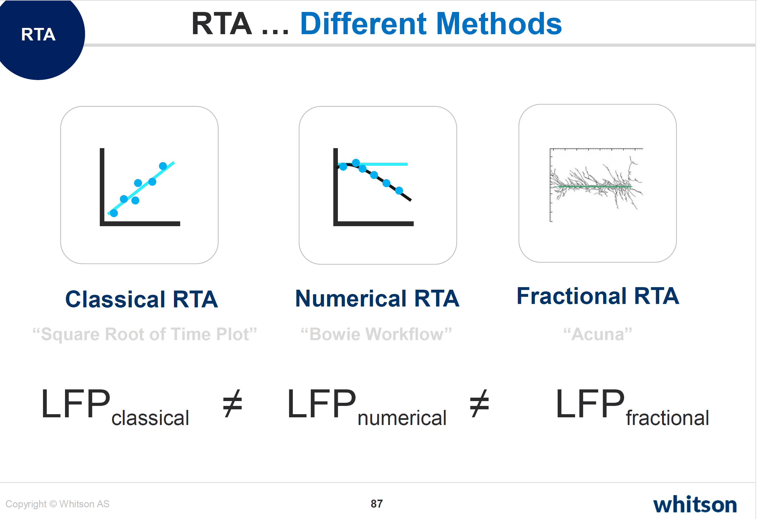
The differences between analytical, fractional and numerical RTA, are due to the following factors:
| Method | Difference |
|---|---|
| Analytical RTA | LFP is derived from single-phase graphical picks from the square root time plot. The equations in Section 1.12 demonstrate the calculation of LFP from the slope. It is important to note that this calculation relies on initial PVT properties. |
| Fractional RTA | LFP is derived using a similar method (graphical slope selection for delta) and is calculated as \(Ak^\delta\), rather than \(Ak^{0.5}\). The governing equations used for the LFP calculation are available here. |
| Numerical RTA | LFP is calculated differently from the two methods above. It is obtained by scaling the LFP of the underlying template model used to generate the simulated finite-acting and infinite-acting stems. The Numerical RTA LFP calculation workflow is available here. |
You can find more information and an example where a numerical model is run and the results are plugged in as input into the analytical RTA solutions in this slide deck here.
6. Constant Flowing Pressure Solution
The constant flowing pressure solution is the opposite of constant rate solution. Instead of having constant rate, it employs variable rate while \(p_{wf}\) is assumed constant.
The workflow of classical RTA is the same for both solutions, the only difference is the equations being used in the calculations. It is worth to mention that there is a factor of \(\pi/2\) difference between the constant rate and constant pressure solutions.
The following equations are applied for constant pressure solution:
6.1. Linear Flow
| Phase | Equation of the Linear Flow |
|---|---|
| Oil | \begin{equation} \label{eq:CP-linear-oil} \frac{\Delta p}{q_o} = \frac{p_i-p_{wf}}{q_o} = \frac{31.3B_o}{h_fx_fn_f\sqrt{k}} \sqrt{\frac{\mu_o}{\phi c_t}} \sqrt{t}+b' \end{equation} |
| Gas | \begin{equation} \label{eq:CP-linear-gas} \frac{\Delta p_p}{q_g} = \frac{p_{p_i}-p_{p_{wf}}}{q_g} = \frac{315.4T_R}{h_fx_fn_f\sqrt{k}} \frac{1}{\sqrt{(\phi\mu_gc_t)_i}} \sqrt{t}+b' \end{equation} |
| Water | \begin{equation} \label{eq:CP-linear-water} \frac{\Delta p}{q_w} = \frac{p_i-p_{wf}}{q_w} = \frac{31.3B_w}{h_fx_fn_f\sqrt{k}} \sqrt{\frac{\mu_w}{\phi c_t}} \sqrt{t}+b' \end{equation} |
| Hydrocarbon | \begin{equation} \label{eq:CR-linear-hc-const-p} \frac{\Delta p}{q_{hc}} = \frac{p_i-p_{wf}}{q_{hc}} = \frac{31.3}{h_fx_fn_f\sqrt{k}} \sqrt{\frac{\mu}{\phi c_t}} \sqrt{t}+b' \end{equation} |
| Liquid | \begin{equation} \label{eq:CR-linear-liq-const-p} \frac{\Delta p}{q_{liq}} = \frac{p_i-p_{wf}}{q_{liq}} = \frac{31.3}{h_fx_fn_f\sqrt{k}} \sqrt{\frac{\mu}{\phi c_t}} \sqrt{t}+b' \end{equation} |
| Total | \begin{equation} \label{eq:CR-linear-total-const-p} \frac{\Delta p}{q_{tot}} = \frac{p_i-p_{wf}}{q_{tot}} = \frac{31.3}{h_fx_fn_f\sqrt{k}} \sqrt{\frac{\mu}{\phi c_t}} \sqrt{t}+b' \end{equation} |
6.2. Slope of straight line
| Phase | Equation of the Slope of Straight Line |
|---|---|
| Oil | \begin{equation} \label{eq:CP-m-oil} m_{CP} = \frac{31.3B_o}{h_fx_fn_f\sqrt{k}} \sqrt{\frac{\mu_o}{\phi c_t}} \end{equation} |
| Gas | \begin{equation} \label{eq:CP-m-gas} m_{CP} = \frac{315.4T_R}{h_fx_fn_f\sqrt{k}} \frac{1}{\sqrt{(\phi\mu_gc_t)_i}} \end{equation} |
| Water | \begin{equation} \label{eq:CP-m-water} m_{CP} = \frac{31.3B_w}{h_fx_fn_f\sqrt{k}} \sqrt{\frac{\mu_w}{\phi c_t}} \end{equation} |
| Hydrocarbon, Liquid, and Total | \begin{equation} \label{eq:CR-m-total-const-p} m_{CR} = \frac{31.3}{h_fx_fn_f\sqrt{k}} \sqrt{\frac{\mu}{\phi c_t}} \end{equation} |
6.3. Linear Flow Parameter
| Phase | Equation of the Linear Flow Parameter |
|---|---|
| Oil | \begin{equation} LFP = A\sqrt{k} = 4\cdot \frac{31.3B_o}{m_{CP}} \sqrt{\frac{\mu_o}{\phi c_t}} \end{equation} |
| Gas | \begin{equation} LFP = A\sqrt{k} = 4\cdot \frac{315.4T_R}{m_{CP}} \sqrt{\frac{1}{(\phi\mu c_t)_i}} \end{equation} |
| Water | \begin{equation} LFP = A\sqrt{k} = 4\cdot \frac{31.3B_w}{m_{CP}} \sqrt{\frac{\mu_w}{\phi c_t}} \end{equation} |
| Hydrocarbon, Liquid, and Total | \begin{equation} LFP = A\sqrt{k} = 4\cdot \frac{31.3}{m_{CR}} \sqrt{\frac{\mu}{\phi c_t}} \end{equation} |
6.4. Distance of Investigation
6.5. Permeability