Chow Pressure Group (CPG)

1. Theory

Chu et al. (2017) showed that there is a relationship between the magnitude of pressure interference (MPI) and the stabilized Chow Pressure Group (CPG) value.

$$\begin{equation} CPG = MPI = \frac{\Delta p}{2\Delta p'} \end{equation}$$

The CPG calculation considers the bottomhole pressure trend before and after a well is put on production (POP). Fig. 1 shows an example of this, where the sloped dashed line represents the pre-POP bottomhole pressure trend and the vertical dashed line represents the actual POP date of the offset well observed in the field. The pressure difference, \(\Delta p\), is the difference between the forecasted "prior" bottomhole pressure trend and the measured bottomhole pressure (that starts when the offset well is put on production).

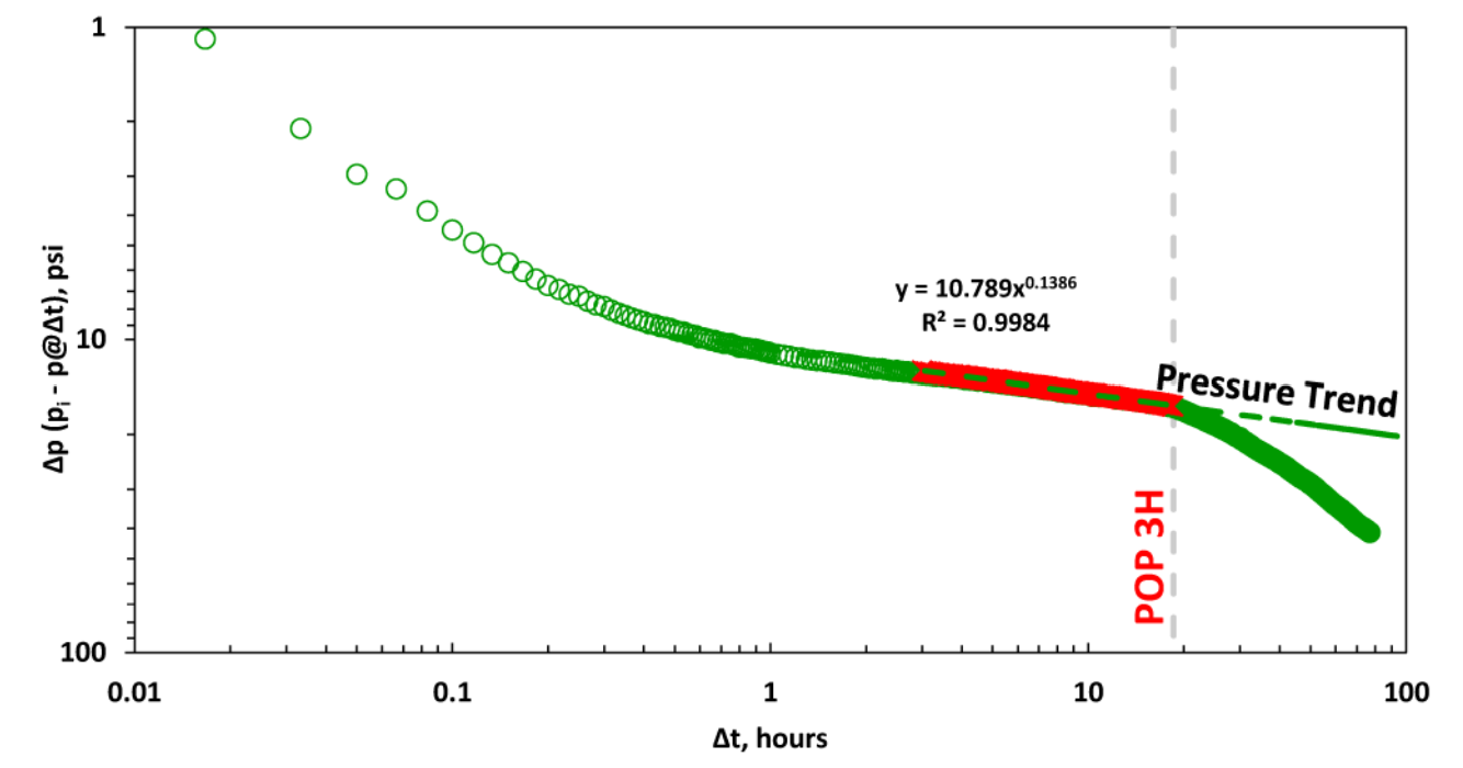
Fig. 1: Example of interference impact when offset well is put on production (POP), Chu et al. (2018).

1.1. Derivative Options

The logarithmic derivative used in well testing applied directly on the \(\Delta p\) data is given by, i.e., $$\begin{equation} \frac{\delta p}{\delta log(t)} = t\frac{\delta p}{\delta t} \end{equation}$$ .

There are three different ways to compute this derivative (\(\Delta p'\)) in whitson⁺:

• The Bourdet Derivative (Bourdet et al., 1989)
• Weighted Central Difference
• Central Difference

1.2. Bourdet Derivative (RECOMMENDED)

The Bourdet derivative is commonly used in well-test analysis (PTA) for identifying flow regimes (Lee et al., 2003) and has similarly found utility in RTA.

1.1.1. Governing Equation

To calculate the Bourdet derivative (Bourdet et al., 1989) at any given point, one point before (left) and one point after (right) are used.

$$\begin{equation} \Delta p' = \frac{\frac{\Delta p_L}{\Delta ln(t)_L}\Delta ln(t)_R + \frac{\Delta p_R}{\Delta ln(t)_R}\Delta ln(t)_L}{\Delta ln(t)_L + \Delta ln(t)_R} \end{equation}$$

1.1.2. Smoothing

The Bourdet approach is illustrated in Fig. 2 and is a way to calculate and smooth the derivative based on a log-cycle window size, L.

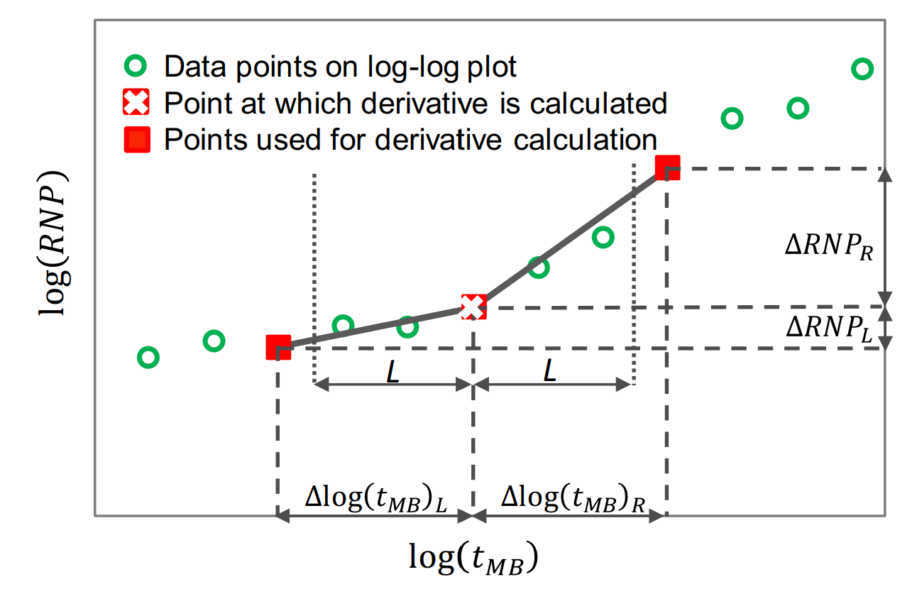
Fig. 2: Illustration of a derivative calculating using the Bourdet method. Image courtesy of Samaneh Moghadam (April, 2020). Modified from Lee et al. (2003).

It differs from a weighted central difference in the way that it uses a constant log-cycle window size (L) on both sides of the point of derivation. A weighted central difference, on the other hand, uses a constant index step size (e.g., i-5 and i+5 for a step size of 5) on each side of the point of derivation. The window size (L) represents the log-cycle fraction used to control the amount of smoothing. Typical values are 0.01 to 0.2. The default L in whitson⁺ is 0.2. The larger the L value, the more smoothing.

The Bourdet algorithm implemented in whitson⁺ was provided by Behnam Zanganeh.

1.2. Weighted Central Difference

The weighted central difference is given by,

$$\begin{equation} \Delta p' = \frac{\frac{\Delta p_L}{\Delta ln(t)_L}\Delta ln(t)_R + \frac{\Delta p_R}{\Delta ln(t)_R}\Delta ln(t)_L}{\Delta ln(t)_L + \Delta ln(t)_R} \end{equation}$$

where the \(L\)-subscript refers to the index on the left with a constant step size, \(S\), i.e., \(i-S\) and the \(R\)-subscript refers to the index to the right with a constant step size, \(S\), i.e., \(i+S\).

1.3. Central Difference

This is the naive implementation, given by three points per derivative for central difference in the following manner:

$$\begin{equation} t\frac{\delta p}{\delta t} = t_i\frac{p_{i+1}-p_{i-1}}{t_{i+1}-t_{i-1}} \end{equation}$$

1.4. Leveraging the Pressure Integral

An alternative approach is to use the pressure integral as the basis to calculate the \(\Delta p\). Here, the \(\Delta p\) is rewritten as an integral as \(\Delta p_{integral}\) - $$\begin{equation} \Delta p_{integral}(t) = \frac{1}{t} \int_0^t \Delta p(t)dt \end{equation}$$ which is implemented in whitson⁺ as $$\begin{equation} \Delta p_{integral}(t_i) = \frac{1}{t_{i}} \sum_{0}^{i} \left(\frac{\Delta p(t_{i}) + \Delta p(t_{i-1}) }{2}\right )(t_i - t_{i-1}) \end{equation}$$ Then, the typical well testing derivative is applied to the \(\Delta p_{integral}\) data as, $$\begin{equation} \frac{\delta p_{integral}}{\delta log(t)} = t\frac{\delta p_{integral}}{\delta t} \end{equation}$$ The integral method preserves the signature of the pressure plot with respect to time while significantly reducing the the noise in the derivatives. This method allows for better stabilization of the derivative values despite noisy pressure data and hence is used for more interpretability in CPG plots.

2. Level of Interference

CPG value	Level of Interference
0	No pressure interference
0-0.5	Weak
0.5-0.8	Moderate
0.8-1	Strong

How is the CPG value related to the slope in \(\Delta p\)?

The \(\Delta p\) slope fit is related to the CPG value and is a favorite way to pick stabilized CPG values as it relies on the analytical relationship between the two and avoids the use of the noisy derivative calculation from field data for an approximated answer.

The derivation of how the calculation of CPG relates to the slope of the \(\Delta p\) data, typically exhibiting power-law behavior, can be shown as follows:

3. Data Requirements and Averaging

To perform this calculation, you only need date (time) and bottomhole pressure data. We recommend averaging the data on a 15 minute basis to remove noise in the data.

4. Example: Drawdown

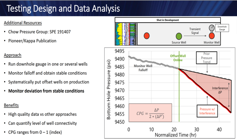
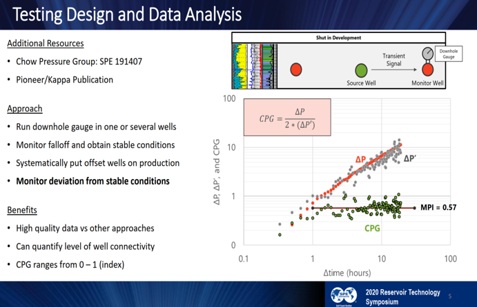
Fig. 3: Drawdown Example (Hart & Ingle, 2020)

5. Example: Buildup

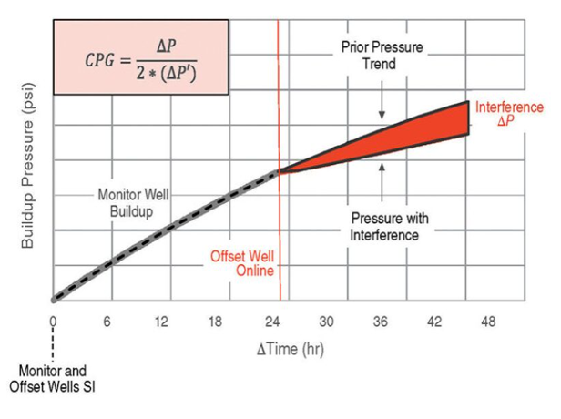
Fig. 4: Drawdown Example (JPT, 2020)

Note

The Chow Pressure Group is not only a convenient way to check the slopes of log-log straight lines, but also means a identify various flow regimes. For example, the slope of 1/2 on the log-log plot may indicate a linear flow regime, which would result in a CPG of one. Likewise, the bilinear flow regime has a slope of 1/4, which would result in a CPG value of 2.

CPG Workflow

Before Getting Started

Recommended Data Size for CPG Tests

CPG datasets can have a much higher frequency than necessary. Datasets may be recorded every second or every few seconds throughout the test, making a dataset more difficult to handle and causing the numerical derivative calculation to become unwieldy.

Rather than uploading high-resolution data, we recommend resampling the dataset externally using pressure increments of 5 to 10 psi. This reduces file size and improves performance. For best results, keep the number of uploaded data rows between 30,000 and 40,000. To learn how to resample your data within whitson⁺, see the resampling section here

Data Truncation

The Truncate Data feature in the Well Testing modules (CPG and DQI) allows users to remove unwanted portions of the dataset and focus the analysis on a specific time range. This is useful for excluding early-time noise, late-time operational changes, or any data outside the period of interest.

Truncation Methods

1. Date-Based Truncation
   Users can manually define the truncation window by selecting a Truncate Start Date and Truncate End Date using the calendar controls. All data outside the selected range is removed.

1. Visual Truncation
   Users can visually select the data range to retain directly on the plot. A black dashed line marks the start of the retained data, and a blue dashed line marks the end. Data before the black line and after the blue line will be deleted.

Create a Project

Here is an example dataset to try it for yourself! Download the CPG Example Dataset here

1. Go to the Projects module in the navigation panel.
2. Click ADD PROJECT in the upper right-corner.
3. Name the project "your name - CPG Example certificate".
4. Click SAVE.
5. Click MASS UPLOAD in the upper-right corner.
6. Upload the CPG Example Dataset Excel file.
7. Click SAVE.
8. All steps are shown in the GIF above.

Chow Pressure Group Analysis

You can analyze the Chow Pressure Group for the monitoring well by navigating to the Chow Pressure Group feature under Well Testing.

Pressure Difference plot

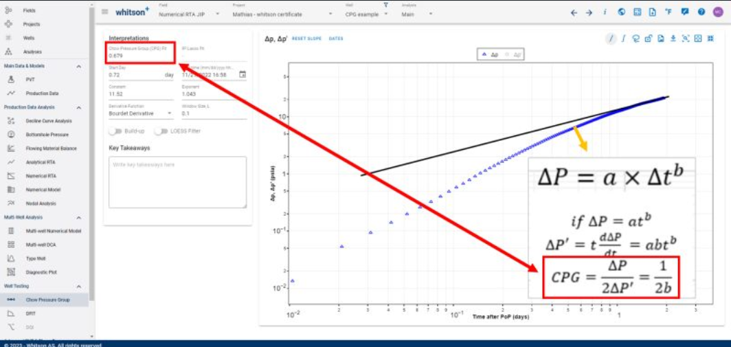
1. Go to the Chow Pressure Group section in the Well Testing module in the navigation panel.
2. On the Pressure Difference plot on the top-left move the CPG fit line (yellow, dashed line) to match the pressure difference data prior to the well put-on-production (POP) date.
3. You can adjust the slope by:
4. Manually moving the fit line on the plot (grab the line at the ends to adjust),
5. Changing the Constant and Exponent of the power-law fit line directly in the input, or
6. Using the lasso tool to fit the pressure data prior to POP and automatically adjust fit line.
7. Adjust the gray, dashed vertical to the date and time when the offset production well was put on production (POP).
8. The difference between the CPG fit and the measured data is plotted, along with its derivative, in the \(\Delta p, \Delta p'\) vs. time plot (bottom-right). Observe how this plot changes as the fit line is adjusted.
9. All steps are shown in the GIF above.

\(\Delta p, \Delta p'\) vs. Time Plot

On the \(\Delta p, \Delta p'\) vs. time plot (bottom-right), you can switch between the derivative calculation techniques mentioned above by selecting 'Derivative Function' from the dropdown menu.
Notice how switching between the different methods and window sizes in the GIF above changes the derivative shape and hence, impacts the CPG values calculated.

Note

Bourdet Derivative and Weighted Central Difference give you the additional option to modify the smoothing window as a log cycle fraction or a step size respectively. Both these methods are higher in accuracy compared to simply using the Central Difference with a fixed step size.

Plot Integral Function

Use the Plot Integral icon in the plot options to recalculate the pressure as an integral and recompute the derivative based on the derivative function selected above. You can also use the LOWESS Filter toggle with an appropriate smoothing window in log cycles to smooth noisy pressure data.

These methods inherently smooth the pressure response and remove additional noise that may be present in the dataset, resulting in a much smoother derivative and CPG plot.

CPG Value

Lastly, on the Chow Pressure Group plot, you can set the final CPG value in three ways:

1. Move the horizontal dashed line to match the average of the CPG values after POP date.
2. Enter a value in the CPG Fit field.
   
3. Select the CPG based on the slope in \(\Delta p\).

This is the CPG value that indicates the level of interference between the production well and the monitoring well.

References

[1] Chu, Weichun , Scott, Kyle , Flumerfelt, Ray , and Chih-Cheng Chen. "A New Technique for Quantifying Pressure Interference in Fractured Horizontal Shale Wells." Paper presented at the SPE Annual Technical Conference and Exhibition, Dallas, Texas, USA, September 2018.

[2] Greenwood, Hart & Ingle, Trevor. "Interference Testing to Advance Appraisal and Development Strategies." Presentation at 2020 Reservoir Technology Symposium.

[3] Jacobs, Trent. "The Chow Pressure Group: Shut-In Wells Offer Case for a New Approach to Interference Testing." JPT 2022.

[4] Bourdet, Dominique, Ayoub, J. A., and Y. M. Plrard. "Use of Pressure Derivative in Well-Test Interpretation." SPE Form Eval 4 (1989): 293–302.

[5] [Christopher R. Clarkson. Unconventional Reservoir Rate-Transient Analaysis. Volume One. Fundamentals, Analysis Methods and Workflow.]

[6] [Lee, J., Rollins, J.B., Spivey, J.P., 2003. Pressure Transient Testing. SPE, Richardson, TX.]