Multiphase Flowing Material Balance

1. Practical use

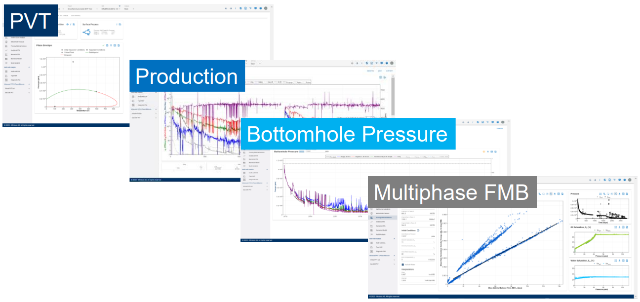
1.1. Multiphase FMB in a Nutshell

Multiphase Flowing Material Balance (MFMB) is a diagnostic plotting method used to analyze multiphase production data.

The method:

• Estimates contacted pore volume ($V_p$) and the corresponding contacted fluid volumes, such as $OOIP$, $OGIP$, and $OWIP$.
• Requires PVT data, production data, flowing bottomhole pressure, and initial reservoir conditions.
• Does not require relative permeability inputs.
• Is primarily interpreted under boundary-dominated flow but can also provide a conservative contacted-volume estimate while the well remains in infinite-acting flow.
• Can be used to constrain or quality-check analytical and numerical RTA interpretations.
• Can be used to evaluate changes in contacted pore volume following a refracture treatment.
• Was developed by Leslie Thompson and Barry Ruddick between 2017 and 2022.

Key benefits:

• MFMB is fast to run and can provide a useful lower-bound estimate of contacted $OOIP$, particularly when production data are noisy or when parameters such as $F_{cd}$ and relative permeability are not yet well constrained in a numerical model.
• The diagnostic response can be used to quality-check the assumed initial water saturation, $S_{wi}$.
• When pressure buildup data are available, the back-calculated average reservoir pressure can be compared with the measured flowing pressure. A physically consistent interpretation should generally satisfy $p_{avg} > p_{wf}$.
• The core MFMB calculation is non-iterative, making it useful for consistently comparing contacted pore volumes across multiple wells.

Interpret MFMB together with other diagnostics

MFMB provides an estimate of the reservoir volume contacted by the well. The result should be interpreted together with pressure behavior, flow-regime diagnostics, PVT consistency, data quality, and other available RTA results.

1.2. Contacted Pore Volume ($V_p$)

MFMB estimates the pore volume that has been hydraulically and dynamically contacted by the well during production.

This contacted pore volume should not be confused with mapped or geologic in-place volume, which is typically larger because it may include reservoir volume that has not contributed to production.

Contacted pore volume is sometimes discussed alongside stimulated rock volume (SRV) and drained rock volume (DRV). However, these terms are not necessarily equivalent:

• Stimulated rock volume generally describes the rock volume affected by hydraulic stimulation.
• Drained rock volume describes the reservoir volume contributing to production.
• Contacted pore volume ($V_p$) is the pore volume inferred from the MFMB production and pressure response.

The contacted $OOIP$, $OGIP$, and $OWIP$ are calculated from $V_p$ using the assumed initial fluid saturations and PVT properties. Therefore, $V_p$, $OOIP$, $OGIP$, and $OWIP$ are related, but they represent different quantities.

1.3. Which Slope Should I Select?

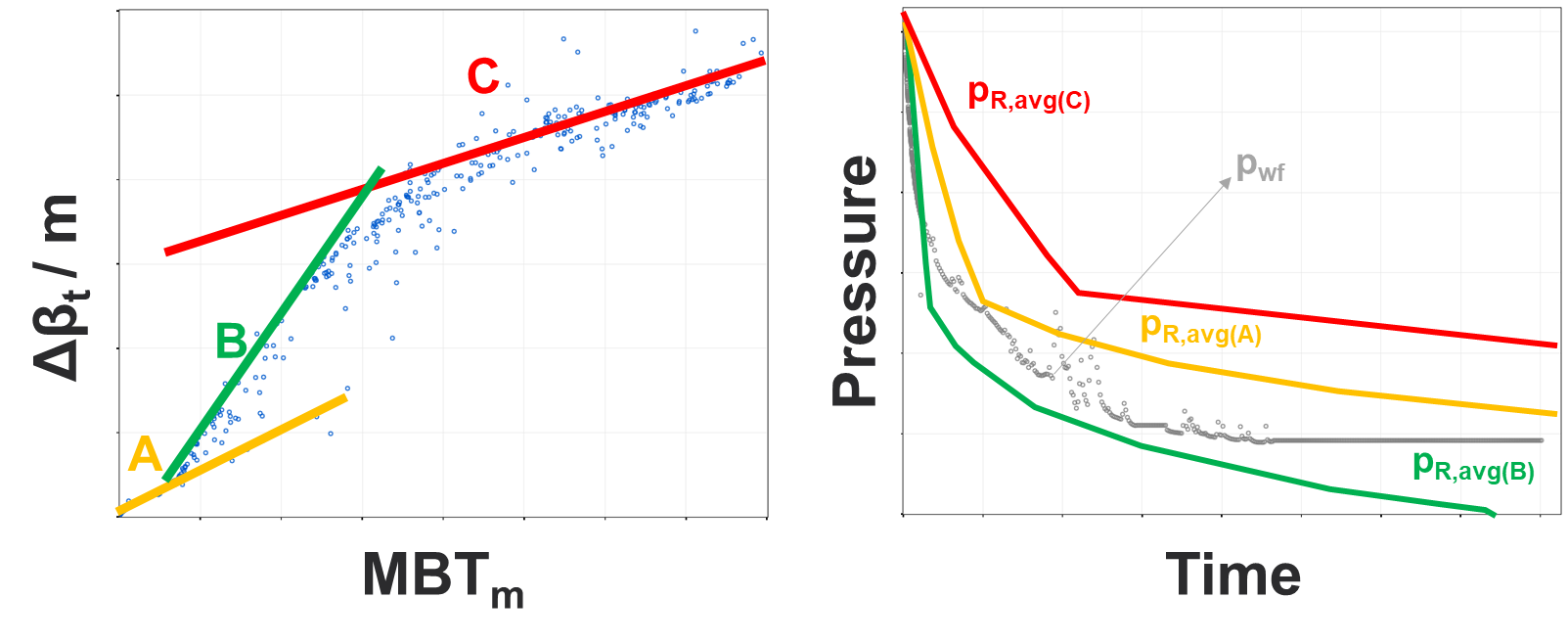
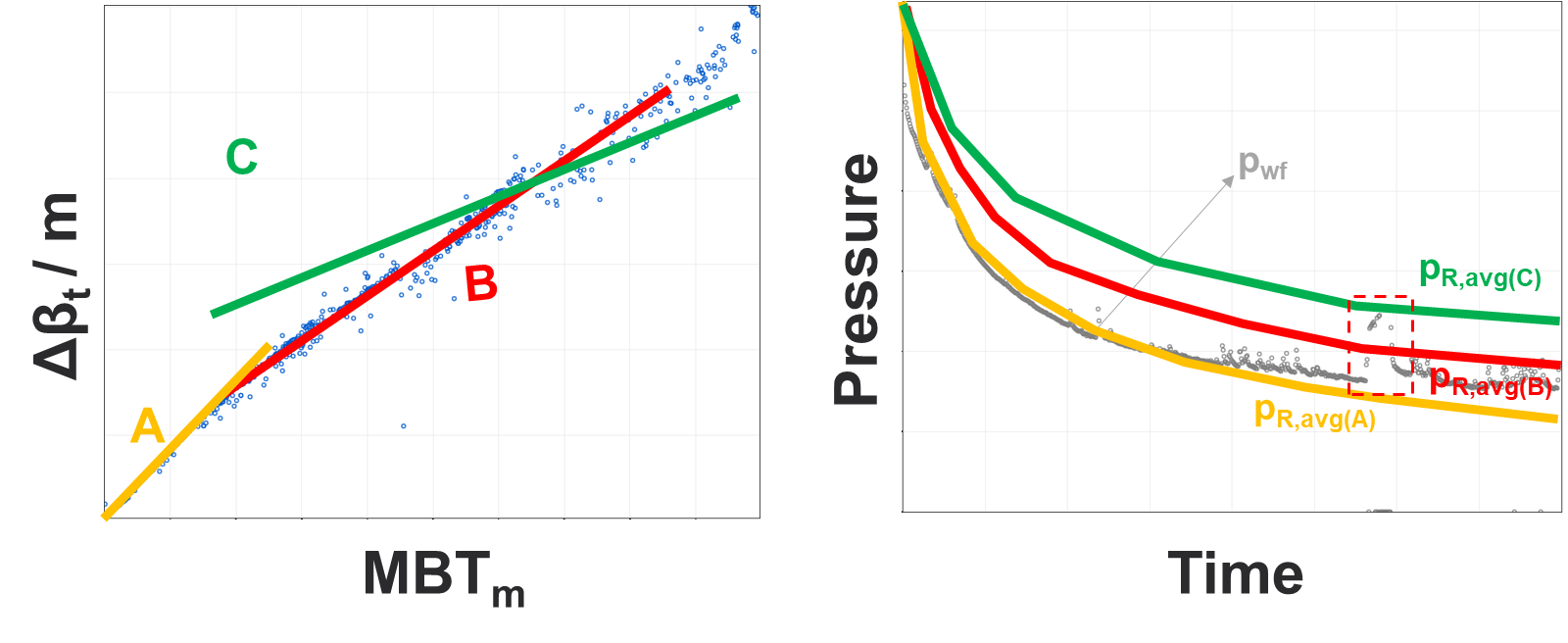
Real field data may exhibit several approximately linear trends on the MFMB diagnostic plot. Each slope corresponds to a different contacted pore-volume estimate.

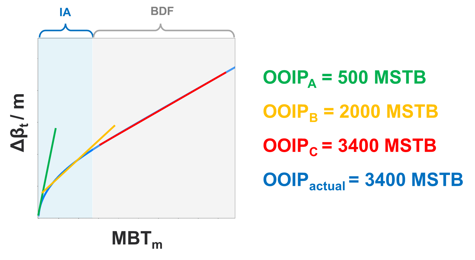
In general, select the shallowest defensible slope because it represents the largest contacted pore volume supported by the observed data.

Each candidate slope produces a different average reservoir pressure ($p_{avg}$) versus time profile. At a minimum, the selected slope should provide a physically consistent pressure response that generally satisfies $p_{avg} > p_{wf}$ throughout the interpreted production period.

The selected trend should also be consistent with:

• The observed depletion behavior.
• Available buildup data.
• Changes in operating conditions.
• Flow-regime interpretation.
• The quality and consistency of the production and pressure data.

1.4. Build-up Data Present

When buildup data are available, adjust the MFMB slope until the back-calculated average reservoir pressure reasonably honors the buildup pressure response.

The slope supported by the buildup data may be shallower—and therefore indicate a larger contacted pore volume—than the slope suggested by depletion data alone.

If a pressure increase is caused by external interference, such as a frac hit or well bashing event, the affected data should generally be excluded from the MFMB trend interpretation.

Distinguish buildup from well interference

A pressure increase caused by shut-in recovery is different from a pressure increase caused by offset-well stimulation or interference. Confirm the operational cause of the pressure response before using it to constrain the MFMB slope.

1.5. What If the Well Is Still Infinite Acting?

If the well remains in infinite-acting flow, the reservoir boundary has not yet been fully observed in the production response. In this case, MFMB can still provide a conservative lower-bound estimate of contacted pore volume and the corresponding contacted $OOIP$, $OGIP$, or $OWIP$.

Analytical or numerical RTA should be used to determine whether the well remains in infinite-acting flow and to provide additional constraints on reservoir geometry and contacted volume.

1.6. Excluding Water from Multiphase FMB

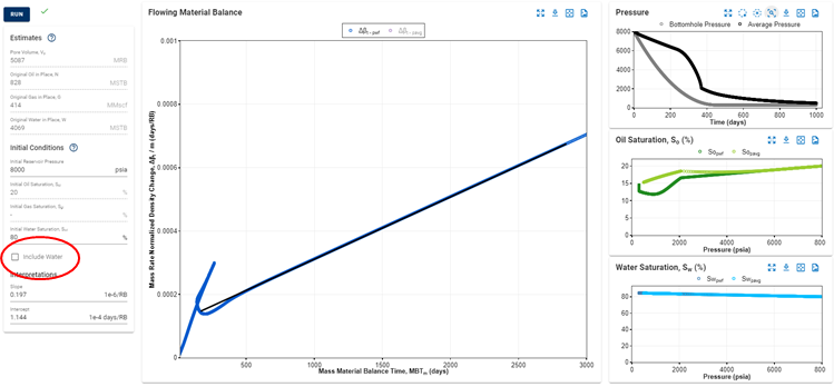
The MFMB calculation includes an option to exclude water production from the analysis. Excluding water will typically produce a more conservative contacted $OOIP$ or $OGIP$ estimate.

This option can be useful for the following reasons:

• It provides a lower contacted hydrocarbon-volume estimate that can be used to bracket the MFMB interpretation.
• Water-rate measurements may contain significant uncertainty. Excluding uncertain water data can produce a cleaner diagnostic trend.
• Some or all of the produced water may originate from a separate water-bearing interval that was contacted during stimulation. In this case, excluding water may provide a more representative analysis of the hydrocarbon-bearing interval.

Use geological and operational context

Water should not be excluded solely to improve the appearance of the MFMB trend. Consider the likely water source, measurement quality, completion geometry, and production history before excluding it.

1.7. MFMB Integral: Reducing Noise

Integral analysis can reduce scatter and make the overall MFMB trend easier to identify. However, integration also smooths the response and may reduce the visibility of shorter-duration diagnostic features.

The MFMB Integral can be displayed from the plot options, as illustrated below.

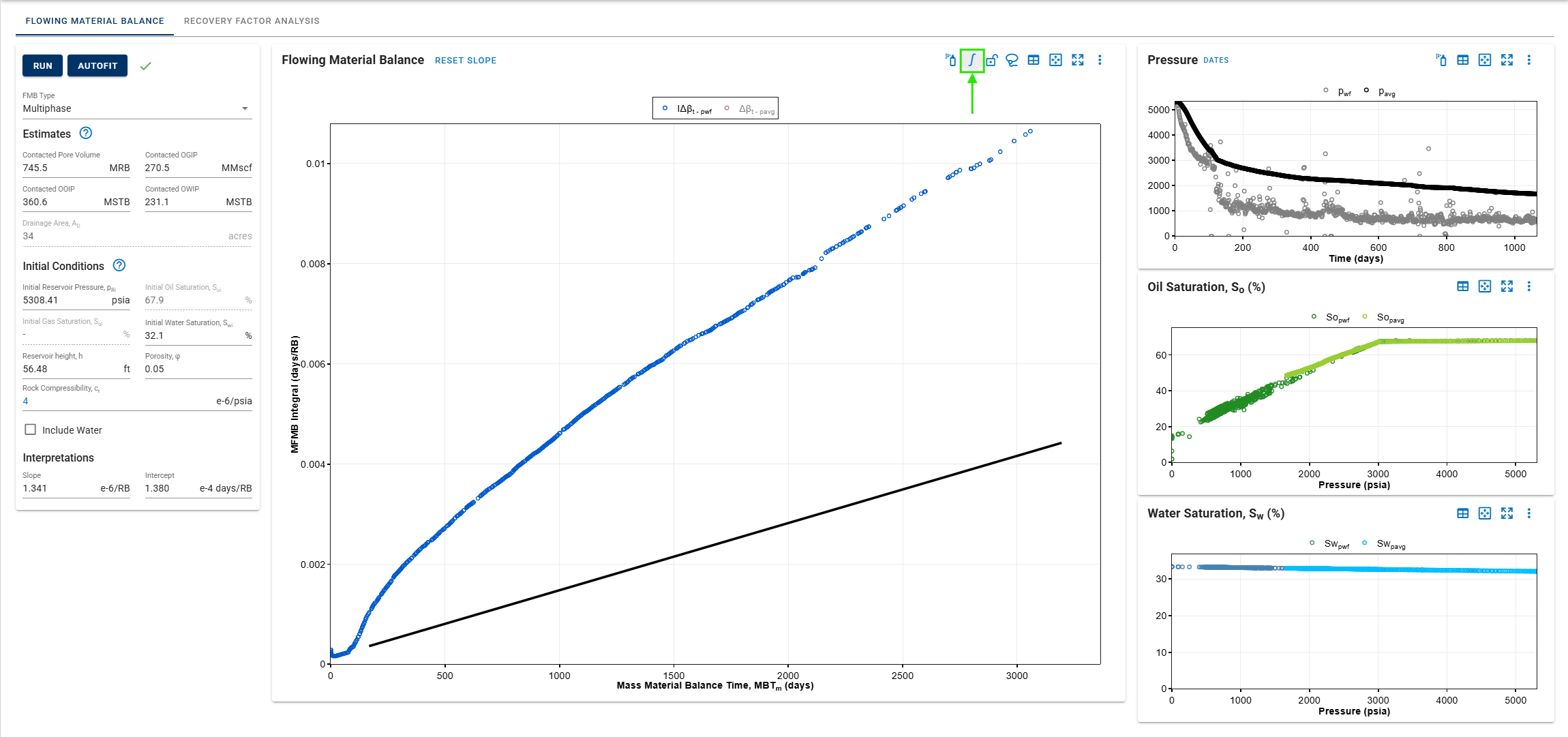
Compare the standard and integral plots

Use the integral plot to identify the overall trend, but compare it with the standard MFMB plot before selecting the final slope. Important changes in reservoir or operating behavior may be less visible after integration.

1.8. Filtering Data Points Across Plots

To filter corresponding data points across the MFMB plots:

1. Select the Spray Filter tool from either the Flowing Material Balance plot or the Pressure plot.
2. Spray a selection around the desired data points.
3. The selected points will be filtered-out in dark yellow across all related plots, including on RTA and Numerical RTA modules.

This feature is useful for investigating specific time intervals, operational changes, pressure behavior, and potential outliers. Also, to remove those data points for being fitted from the Autofit.

1.9. Autofit

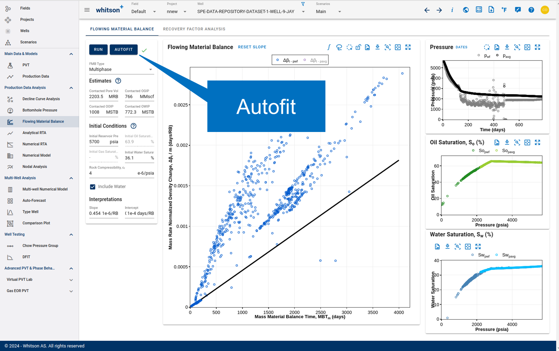
The MFMB Autofit feature estimates the slope of the straight-line portion of the diagnostic plot. The selected slope is used to calculate contacted pore volume.

Autofit evaluates two candidate trends:

• A straight-line fit through data points where flowing bottomhole pressure, $p_{wf}$, is above saturation pressure, $p_{sat}$.
• A straight-line fit through the final 20% of the observed production-history data points.

The shallower of the two candidate slopes is selected, corresponding to the larger contacted pore-volume estimate.

whitson⁺ provides two Autofit modes:

1. Standard Autofit

   Performs a straight-line fit using the two criteria described above. This mode does not impose the additional constraint that the calculated average reservoir pressure must be greater than the flowing bottomhole pressure.

2. Autofit with $p_{avg} > p_{wf}$ Criteria

   Starts from the automatically selected straight-line fit and iteratively increases the contacted pore volume when the calculated pressure response does not satisfy the physical pressure constraint. The pore volume can be adjusted up to 10 times until at least 95% of the evaluated data points satisfy: $p_{avg} > p_{wf}$

Autofit is a starting point

Autofit provides a consistent initial interpretation, but the result should still be reviewed manually. Consider pressure buildup data, saturation pressure, operational changes, interference events, flow-regime behavior, and overall data quality before accepting the final contacted pore volume.

2. Multiphase FMB: Theory

2.1. Governing Equation

The multiphase flowing material balance equation is written as:

$$\begin{equation} \label{eq:multiphase-FMB-governing} \frac{\beta_i-\gamma\bar{\beta}}{\dot{m}(t)}=\frac{1}{V_p}{MBT}_M+\frac{1}{b_M} \end{equation}$$

This equation has the form of a straight line: $y=ax+b$, where:

$$\begin{equation} y=\frac{\beta_i-\gamma\bar{\beta}}{\dot{m}(t)} \end{equation}$$

$$\begin{equation} x={MBT}_M \end{equation}$$

$$\begin{equation} a=\frac{1}{V_p} \end{equation}$$

$$\begin{equation} b=\frac{1}{b_M} \end{equation}$$

Therefore, the slope of the straight-line trend is inversely proportional to the contacted pore volume:

$$\begin{equation} V_p=\frac{1}{a} \end{equation}$$

A shallower slope consequently corresponds to a larger contacted pore volume.

2.2. MFMB Integral

The multiphase FMB diagnostic plot can be noisy when applied to field data. The MFMB Integral reduces data scatter and makes the underlying straight-line trend easier to identify.

For convenience, define the left-hand side of the governing equation at time step $i$ as: $$\begin{equation} \label{eq:multiphase-FMB-i} MFMB_i = \frac{\beta_i-\gamma\bar{\beta}_i}{\dot{m}_i} \end{equation}$$ Define mass material balance time at time step $i$ as:

$$\begin{equation} \label{eq:matbaltime} t_i={MBT}_{M,i} \end{equation}$$

The MFMB Integral is defined as:

$$\begin{equation} \label{eq:multiphase-FMB-integral-continuous} MFMB_{\mathrm{integral},i} = \frac{2}{t_i} \int_{0}^{t_i} MFMB(t)\,dt \end{equation}$$

Using the trapezoidal rule, the integral can be evaluated from discrete production data as:

$$\begin{equation} \label{eq:multiphase-FMB-integral} MFMB_{\mathrm{integral},i} = \frac{1}{t_i} \sum_{j=1}^{i} \left(MFMB_j+MFMB_{j-1}\right) \left(t_j-t_{j-1}\right) \end{equation}$$

The integral is multiplied by 2 and divided by $t_i$ so that the slope of the transformed diagnostic plot remains equal to $1/V_p$.

To demonstrate this, consider a linear function: $f(x)=ax+b$

Integrating from 0 to $x$ gives:

$$\begin{equation} \int_{0}^{x}f(u)\,du = \frac{1}{2}ax^2+bx \end{equation}$$

Multiplying the integral by $2/x$ gives:

$$\begin{equation} \frac{2}{x}\int_{0}^{x}f(u)\,du = ax+2b \end{equation}$$

Therefore, the integral transformation preserves the original slope ($a$) while changing the intercept from $b$ to $2b$. Because the slope remains $1/V_p$, the contacted pore volume can still be calculated directly from the MFMB Integral plot.

Effect of integration

The MFMB Integral reduces noise but also smooths short-duration changes in the diagnostic response. Use the integral plot to identify the overall trend, but compare it with the standard MFMB plot before selecting the final slope.

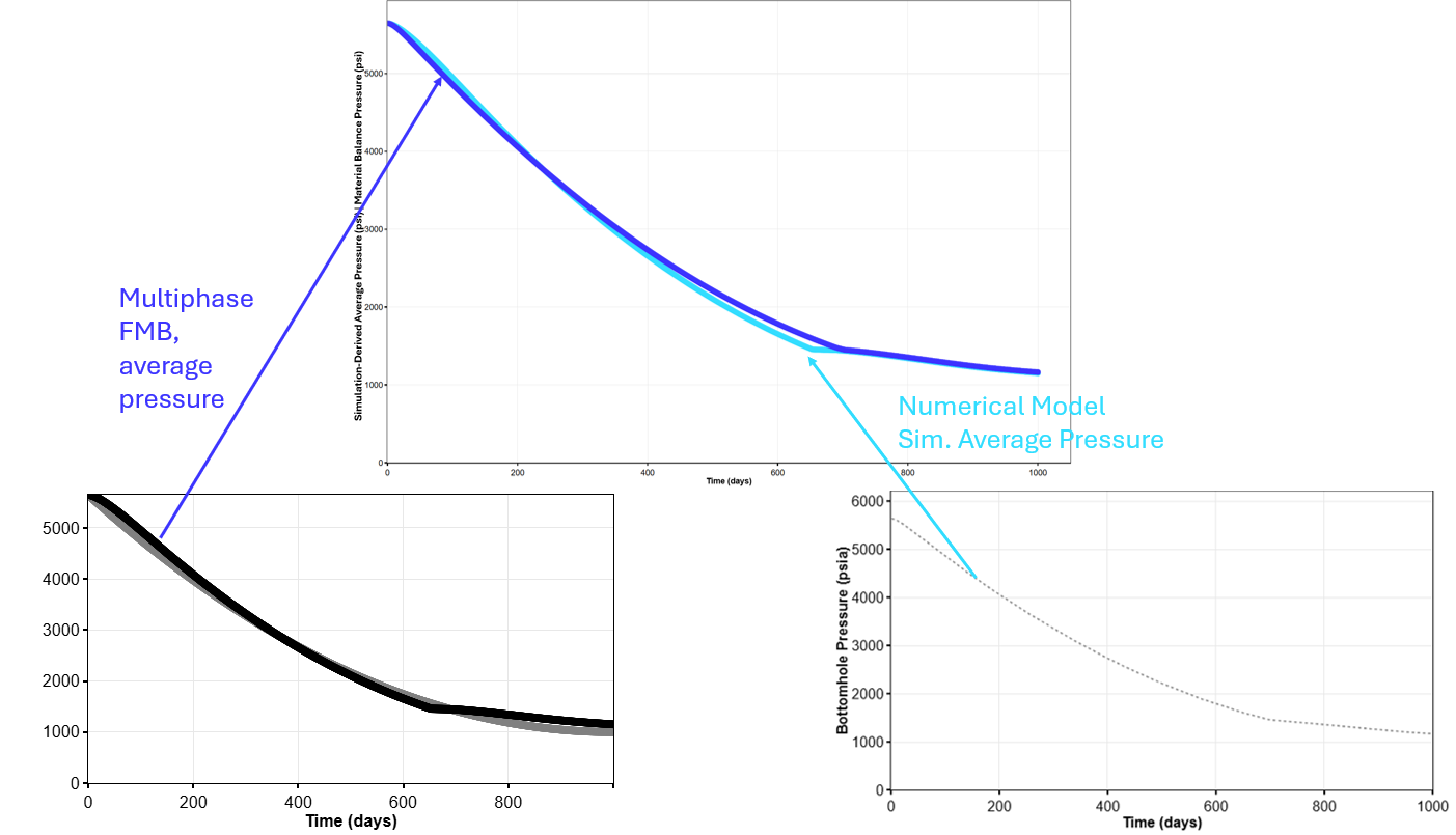
2.3. Simulation vs. FMB Average Pressure

There is an important distinction between the average reservoir pressure calculated from a numerical simulation model and the material balance pressure back-calculated by FMB.

The simulation-derived average pressure is calculated from the pressure distribution across the grid cells using the averaging or weighting method defined by the simulator, such as pore-volume or hydrocarbon-pore-volume weighting.

In contrast, the FMB average pressure represents the equivalent pressure of a single, well-mixed tank containing the same total fluid mass. It is obtained from the material balance relationship and accounts for pressure-dependent fluid properties and compressibility, including the gas $p/z$ behavior.

The two pressure estimates are equal only when the reservoir behaves as a sufficiently uniform tank with negligible pressure and composition gradients. In real reservoirs, pressure depletion, multiphase behavior, and compositional variation can cause the two values to differ. These differences may become particularly noticeable during transient flow, pressure buildup, or shut-in periods.

3. Multiphase FMB: Detailed Theory

The Multiphase Flowing Material Balance (MFMB) module is based on the workflow proposed by Thompson and Ruddick in URTeC 2022.

The workflow accounts for phase and saturation changes during multiphase production that are not captured by conventional single-phase flowing material balance methods. Unlike other multiphase FMB approaches, this method does not require explicit relative permeability relationships or pseudopressure functions.

The method is based on mass conservation and uses production data, PVT properties, and initial reservoir conditions to estimate the contacted pore volume and corresponding original fluids in place.

Classical single-phase FMB combines pseudo-steady-state flow theory with material balance. The multiphase workflow relies on a similar assumption: during constant-rate pseudo-steady-state flow, the mixture density throughout the contacted reservoir volume declines at approximately the same rate.

Why does the multiphase FMB method not require pressure-dependent permeability inputs?

“All transport-dependent terms (permeability, relative permeability, etc.) are built into the rates. They never appear explicitly.”

— Leslie Thompson

The multiphase FMB governing equation is:

$$\begin{equation} \label{eq:multiphase-FMB} \frac{\beta_i-\gamma\bar{\beta}}{\dot{m}(t)} = \frac{1}{V_p}{MBT}_M+\frac{1}{b_M} \end{equation}$$

where $\beta$ is the mixture density, expressed in lbm/bbl:

$$\begin{equation} \label{eq:Mixture-Density} % lbm/bbl \beta(t)=5.615\rho_{osc}\left(\frac{S_o}{B_o}+\frac{S_gR_v}{B_g}\right)_{t}+1000\rho_{gsc}\left(\frac{S_oR_s}{B_o}+\frac{S_g}{B_g}\right)_{t}+5.615\rho_{wsc}\left(\frac{S_w}{B_w}\right)_{t} \end{equation}$$

The pore-volume correction factor ($\gamma$) is the ratio of the pore volume at the pressure of interest to the initial pore volume:

$$\begin{equation} \label{eq:gamma} \gamma=\frac{V_p}{V_{pi}}=\exp\left(-\int_p^{p_i}c_r\left(p\right)\,dp\right) \end{equation}$$

where $c_r(p)$ is the pressure-dependent rock compressibility.

The total mass production rate ($\dot{m}$), is expressed in lbm/d and is defined as:

$$\begin{equation} \label{eq:Total-Mass-Production} % lbm/d \dot{m}(t)=5.615\rho_{osc}q_o(t)+1000\rho_{gsc}q_g(t)+5.615\rho_{wsc}q_w(t) \end{equation}$$

Mass material balance time (${MBT}_M$) is expressed in days and is defined as:

$$\begin{equation} \label{eq:Mass-Material-Balance} % day {MBT}_M(t)=\frac{M_T(t)}{\dot{m}(t)} \end{equation}$$

where $M_T(t)$ represents the total cumulative mass of oil, gas, and water produced from the reservoir:

$$\begin{equation} \label{eq:Cumulative-Mass-Produced-Oil} % lbm M_o(t)=5.615\rho_{osc}N_p(t) \end{equation}$$

$$\begin{equation} \label{eq:Cumulative-Mass-Produced-Gas} % lbm M_g(t)=1000\rho_{gsc}G_p(t) \end{equation}$$

$$\begin{equation} \label{eq:Cumulative-Mass-Produced-Water} % lbm M_w(t)=5.615\rho_{wsc}W_p(t) \end{equation}$$

$$\begin{equation} \label{eq:Cumulative-Mass-Produced-Total} % lbm M_T(t)=M_o(t)+M_g(t)+M_w(t) \end{equation}$$

The subscript $i$ represents the initial reservoir condition, while the overbar represents an average reservoir condition. Subscripts $o$, $g$, and $w$ represent oil, gas, and water properties, respectively.

The terms $\rho_{osc}$, $\rho_{gsc}$, and $\rho_{wsc}$ represent phase densities at standard conditions. The variables $S$, $B$, and $q$ represent saturation, formation volume factor, and production rate, respectively. $V_p$ is the contacted pore volume, while $N_p$, $G_p$, and $W_p$ are cumulative oil, gas, and water production.

According to Eq. \eqref{eq:multiphase-FMB}, plotting the mass-rate-normalized mixture-density difference, $\frac{\beta_i-\gamma\bar{\beta}}{\dot{m}(t)}$ against mass material balance time (${MBT}_M$) produces a straight-line trend with:

$$\begin{equation} \text{Slope}=\frac{1}{V_p} \end{equation}$$

and:

$$\begin{equation} \text{Intercept}=\frac{1}{b_M} \end{equation}$$

Therefore, the contacted pore volume is calculated as:

$$\begin{equation} V_p=\frac{1}{\text{Slope}} \end{equation}$$

The intercept represents the multiphase productivity term. A finite productivity index produces a positive intercept on the MFMB diagnostic plot.

Once the contacted pore volume has been determined, the corresponding original fluids in place can be calculated using the following relationships:

$$\begin{equation} \label{eq:OIP} % STB OIP = V_p\left(\frac{S_{o}}{B_{o}}+\frac{S_{g}R_{v}}{B_{g}}\right)_i \end{equation}$$

$$\begin{equation} \label{eq:GIP} % Mscf GIP = V_p\left(\frac{S_{o}R_{s}}{B_{o}}+\frac{S_{g}}{B_{g}}\right)_i \end{equation}$$

$$\begin{equation} \label{eq:WIP} % STB WIP = V_p\left(\frac{S_{w}}{B_{w}}\right)_i \end{equation}$$

The component concentrations of oil, gas, and water, denoted by $\zeta_o$, $\zeta_g$, and $\zeta_w$, are defined as:

$$\begin{equation} \label{eq:Component-Concentration-Oil} % (STB/bbl) \zeta_{o}=\frac{S_o}{B_o}+\frac{S_gR_v}{B_g} \end{equation}$$

$$\begin{equation} \label{eq:Component-Concentration-Gas} % (Mscf/bbl) \zeta_{g}=\frac{S_oR_s}{B_o}+\frac{S_g}{B_g} \end{equation}$$

$$\begin{equation} \label{eq:Component-Concentration-Water} % (STB/bbl) \zeta_{w}=\frac{S_w}{B_w} \end{equation}$$

Consider mass conservation within the reservoir volume immediately adjacent to the producing wellbore:

1. At early time, the cumulative producing-fluid ratios of the reservoir and near-wellbore region are identical because production originates primarily from the near-wellbore region.
2. At later time, the cumulative producing-fluid ratios of the reservoir and near-wellbore region are assumed to remain approximately equal.

Using these assumptions, the following cumulative production-ratio relationships can be derived:

$$\begin{equation} \label{eq:Oil-Gas-Ratio} % STB/Mscf OGR(t)=\frac{N_p}{G_p}=\frac{\left(\frac{S_o}{B_o}+\frac{S_gR_v}{B_g}\right)_{i}-\gamma\left(\frac{S_o}{B_o}+\frac{S_gR_v}{B_g}\right)_{well}}{\left(\frac{S_oR_s}{B_o}+\frac{S_g}{B_g}\right)_{i}-\gamma\left(\frac{S_oR_s}{B_o}+\frac{S_g}{B_g}\right)_{well}}=\frac{\zeta_{oi}-\gamma\left(\frac{S_o}{B_o}+\frac{S_gR_v}{B_g}\right)_{well}}{\zeta_{gi}-\gamma\left(\frac{S_oR_s}{B_o}+\frac{S_g}{B_g}\right)_{well}} \end{equation}$$

$$\begin{equation} \label{eq:Water-Gas-Ratio} % STB/Mscf WGR(t)=\frac{W_p}{G_p}=\frac{\left(\frac{S_w}{B_w}\right)_{i}-\gamma\left(\frac{S_w}{B_w}\right)_{well}}{\left(\frac{S_oR_s}{B_o}+\frac{S_g}{B_g}\right)_{i}-\gamma\left(\frac{S_oR_s}{B_o}+\frac{S_g}{B_g}\right)_{well}}=\frac{\zeta_{wi}-\gamma\left(\frac{S_w}{B_w}\right)_{well}}{\zeta_{gi}-\gamma\left(\frac{S_oR_s}{B_o}+\frac{S_g}{B_g}\right)_{well}} \end{equation}$$

$OGR$ is the cumulative producing oil-gas ratio in STB/Mscf, while $WGR$ is the cumulative producing water-gas ratio in STB/Mscf.

Rearranging Eqs. \eqref{eq:Oil-Gas-Ratio} and \eqref{eq:Water-Gas-Ratio} allows the phase saturations to be calculated:

$$\begin{equation} \label{eq:Oil-Saturation} % (-) S_o=-\frac{B_o\left[\Gamma_o+\zeta_{oi}\left(B_g+B_wWGR\right)-\zeta_{gi}\left(B_gOGR+B_wWGRR_v\right)\right]}{\gamma\left[B_g\left(OGR R_s-1\right)-B_o\left(OGR-R_v\right)+B_wWGR\left(R_sR_v-1\right)\right]} \end{equation}$$

$$\begin{equation} \label{eq:Water-Saturation} % (-) S_w=-\frac{B_w\left[\Gamma_w+\zeta_{wi}\left(B_g\left(1-OGRR_s\right)+B_o\left(OGR-R_v\right)\right)\right]}{\gamma\left[B_g\left(OGR R_s-1\right)-B_o\left(OGR-R_v\right)+B_wWGR\left(R_sR_v-1\right)\right]} \end{equation}$$

$$\begin{equation} \label{eq:Gas-Saturation} % (-) S_g=1-S_w-S_o \end{equation}$$

where: $$\begin{equation} \label{eq:Gamma-constanta} \Gamma_o=\left(\gamma-\zeta_{wi}B_w\right)\left(OGR-R_v\right) \end{equation}$$

$$\begin{equation} \label{eq:Gamma-w-constanta} \Gamma_w=\left[\gamma\left(1-R_sR_v\right)+\zeta_{gi}\left(B_oR_v-B_g\right)+\zeta_{oi}\left(B_gR_s-B_o\right)\right]WGR \end{equation}$$

Total compressibility accounts for the compressibility of each fluid phase present in the reservoir, together with rock compressibility:

$$\begin{equation} \label{eq:ct} % 1/psia c_t=c_gS_g+c_oS_o+c_wS_w+c_r \end{equation}$$

where $c_g$, $c_o$, $c_w$, and $c_r$ represent gas, oil, water, and rock compressibility, respectively.

Default rock compressibility in whitson⁺

The default values used in the software are:

$$c_r=4\times10^{-6}\ \text{psi}^{-1}$$

and:

$$c_w=2.8\times10^{-6}\ \text{psi}^{-1}$$

The complete derivation provided by the authors is available here.

For additional details, refer to URTeC-3718045 by Thompson and Ruddick.

3.1. Intercept on the Multiphase FMB Plot

A negative MFMB intercept is not physically expected under normal reservoir depletion.

The theoretical minimum intercept is zero, corresponding to the limiting case in which the contacted reservoir behaves as a perfectly mixed tank. The average-pressure trend therefore represents the theoretical lower bound of the MFMB diagnostic response.

If the observed wellbore data fall below this limit, possible causes include:

• External pressure support.
• Offset-well interference or a frac hit.
• Inconsistent pressure or production data.
• Selection of an inappropriate linear trend.
• Unaccounted changes in operating conditions.

For positive intercepts, the calculated recovery factors are generally less sensitive to the exact intercept than to the selected MFMB slope. However, increasing the intercept typically produces a slightly lower calculated recovery factor.

Prioritize the slope interpretation

The MFMB slope controls the contacted pore-volume estimate and usually has a greater influence on the interpretation than the intercept. Both parameters should nevertheless be physically reasonable and consistent with the observed pressure response.

3.2. Note on a Slightly Compressible Fluid by Leslie Thompson

For a slightly compressible fluid with a small, constant compressibility, produced at a constant rate during pseudo-steady-state flow, the pressure decline rate is constant.

For this case, density can be approximated as:

$$\begin{equation} \label{eq:rho} \rho-\rho_{sc}=\rho_{sc}c\left(p-p_{sc}\right) \end{equation}$$

where $c$ is fluid compressibility and the subscript $sc$ represents standard conditions.

Differentiating this relationship with respect to time gives:

$$\begin{equation} \label{eq:dpdt2} \frac{\partial p}{\partial t} = \frac{1}{\rho_{sc}c} \frac{\partial \rho}{\partial t} \end{equation}$$

Therefore, for a slightly compressible fluid, the condition:

$$\begin{equation} \frac{\partial p}{\partial t}=\text{constant}\ \end{equation}$$

For these systems, rate-normalized pressure drop is accepted as a linear function of material balance time during boundary-dominated flow. Because pressure and density are directly related for a slightly compressible fluid, mass-rate-normalized density change is similarly expected to be a linear function of mass material balance time.

Multiphase depletion is considerably more complex. Local depletion depends on pressure and fluid composition, both of which may change continuously and differently throughout the reservoir.

It may therefore appear surprising that a simplified, single-tank representation can capture enough of the reservoir depletion behavior to support a material balance interpretation. However, the classical Schilthuis material balance method has historically demonstrated that a simplified tank model can provide a useful representation of global reservoir behavior.

The proposed multiphase method follows the same principle. It does not reproduce the detailed local behavior at every point in the reservoir. Instead, it captures enough of the governing physics to provide a practical approximation of the reservoir's global depletion response.

4. Workflow

The multiphase FMB calculation is performed using the following workflow:

1. Calculate the initial fluid properties from the provided PVT data:

   • Initial oil formation volume factor ($B_{oi}$)
   • Initial gas formation volume factor ($B_{gi}$)
   • Initial water formation volume factor ($B_{wi}$)
   • Initial solution gas-oil ratio ($R_{si}$)
   • Initial solution condensate-gas ratio ($R_{vi}$)

   Using these properties and the initial fluid saturations, calculate the initial mixture density ($\beta_i$) with Eq. \eqref{eq:Mixture-Density}.

2. For each production time step, calculate the following:

   • Cumulative oil, gas, and water production: $N_p(t)$, $G_p(t)$, and $W_p(t)$
   • Mass production rate ($\dot{m}(t)$) using Eq. \eqref{eq:Total-Mass-Production}
   • Cumulative produced oil, gas, and water masses using Eqs. \eqref{eq:Cumulative-Mass-Produced-Oil}, \eqref{eq:Cumulative-Mass-Produced-Gas}, and \eqref{eq:Cumulative-Mass-Produced-Water}
   • Total produced mass ($M_T(t)$) using Eq. \eqref{eq:Cumulative-Mass-Produced-Total}
   • Mass material balance time (${MBT}_M(t)$) using Eq. \eqref{eq:Mass-Material-Balance}
   • Cumulative producing oil-gas ratio ($OGR(t)$) and water-gas ratio ($WGR(t)$)
   • Fluid properties at the applicable average reservoir pressure: $B_o(t)$, $B_g(t)$, $B_w(t)$, $R_s(t)$, and $R_v(t)$
   • Rock pore-volume correction factor, $\gamma(t)$, using Eq. \eqref{eq:gamma}
   • Oil, water, and gas saturations, $S_o(t)$, $S_w(t)$, and $S_g(t)$, using Eqs. \eqref{eq:Oil-Saturation}, \eqref{eq:Water-Saturation}, and \eqref{eq:Gas-Saturation}
   • Average mixture density ($\bar{\beta}(t)$) using Eq. \eqref{eq:Mixture-Density}
   • Mass-rate-normalized mixture-density difference:

   $$\frac{\Delta\beta(t)}{\dot{m}(t)} = \frac{\beta_i-\gamma(t)\bar{\beta}(t)} {\dot{m}(t)}$$

3. Create the multiphase FMB diagnostic plot with:

   • Mass material balance time (${MBT}_M$) on the x-axis
   • Mass-rate-normalized mixture-density difference ($\frac{\beta_i-\gamma\bar{\beta}}{\dot{m}(t)}$) on the y-axis

4. Identify the appropriate straight-line trend and determine its slope and intercept.

   According to Eq. \eqref{eq:multiphase-FMB}, the contacted pore volume is:

   $$V_p=\frac{1}{\text{Slope}}$$

   expressed in reservoir barrels.

5. Calculate the corresponding original fluids in place using:

   • Eq. \eqref{eq:OIP} for oil in place
   • Eq. \eqref{eq:GIP} for gas in place
   • Eq. \eqref{eq:WIP} for water in place

5. Refracs

A refrac, or refracturing treatment, is an additional hydraulic fracturing operation performed on a well that has previously been stimulated.

During a refrac treatment, high-pressure fluid is pumped into the well to create new fractures, reopen existing fractures, or reconnect portions of the fracture network that have become less productive after the initial production period.

A successful refrac may contact previously unstimulated reservoir volume with higher remaining pressure. Refracturing can therefore increase production and may provide a cost-effective alternative to drilling a new well.

5.1. Refrac Analysis Workflows

There are two primary refrac-analysis applications:

1. Evaluate an existing refrac

   To evaluate a refrac that has already been completed, use the MFMB workflow described in the following section. This approach was applied by Young et al. (2023) to evaluate 46 refractured wells in the Eagle Ford using whitson⁺.

2. Estimate uplift from a planned refrac

   To predict the production uplift from a refrac that has not yet been performed, use the Numerical Model refrac workflow. See Refrac Analysis: Estimating Uplift on Planned Refracs.

5.1.1. Existing Refrac Analysis Workflow

Use the following workflow to evaluate whether an existing refrac increased the contacted reservoir volume:

1. Define the initial reservoir conditions, initialize the PVT model, and calculate flowing bottomhole pressure.
2. Divide the production history into pre-refrac and post-refrac periods.
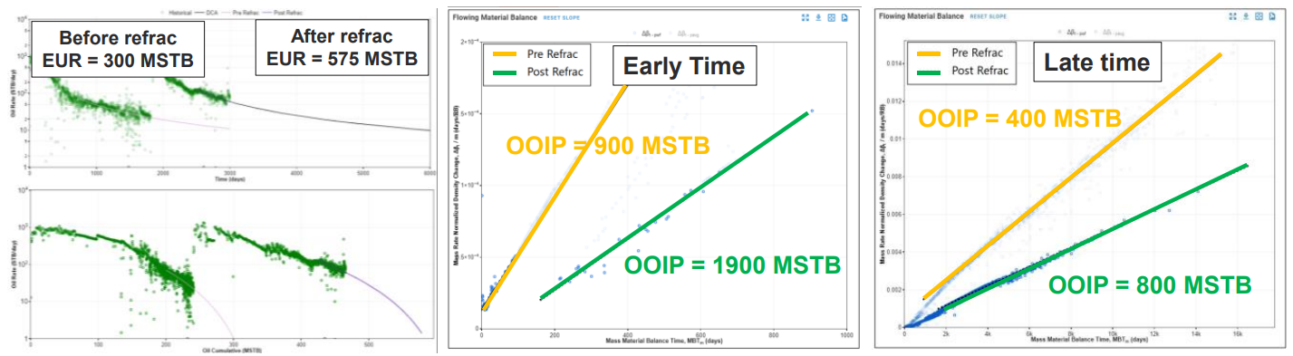
3. On the MFMB diagnostic plot, identify comparable early-time and late-time linear trends for both periods, pre-refrac and post-refrac.
4. Calculate the contacted $OOIP$ from each selected MFMB slope.
5. Compare the pre-refrac and post-refrac contacted $OOIP$ estimates separately for the early-time and late-time interpretations.
6. Estimate the refrac-related increase in contacted $OOIP$ from the two comparisons.

Use consistent assumptions

Use consistent PVT properties, initial reservoir conditions, pressure calculations, and data-treatment assumptions when comparing the pre-refrac and post-refrac periods.

5.1.2. Successful Refrac Response

A successful refrac should produce a larger post-refrac contacted $OOIP$ estimate than the corresponding pre-refrac estimate.

Ideally, an increase should be observed in both the early-time and late-time MFMB slope interpretations.

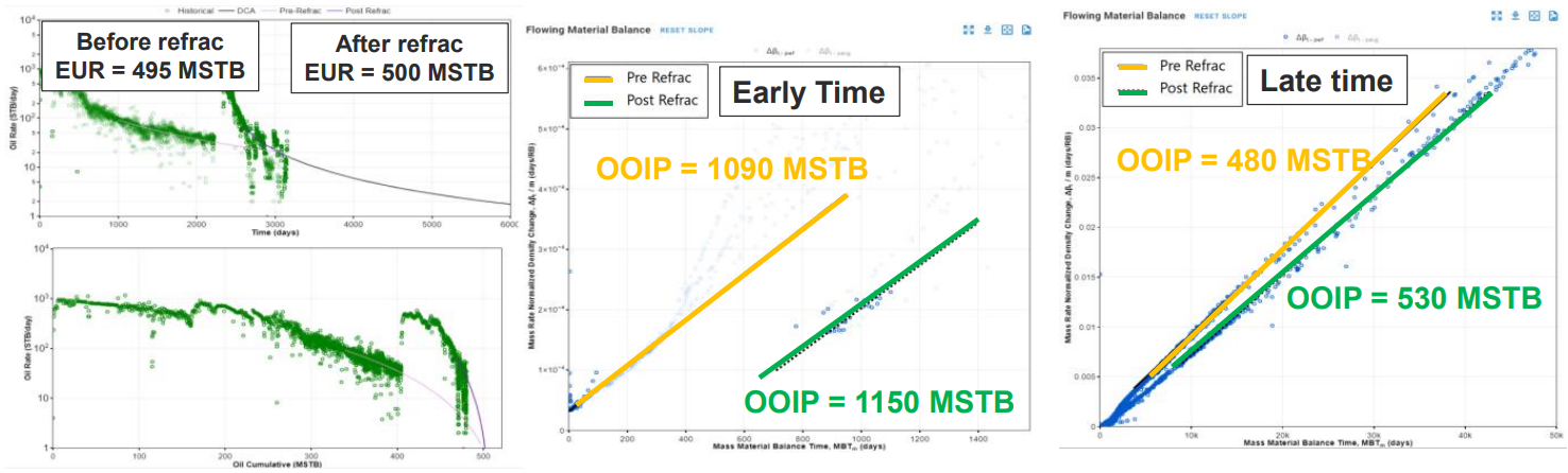
5.1.3. Unsuccessful Refrac Response

An unsuccessful refrac may show little or no increase in contacted $OOIP$. In some cases, the post-refrac estimate may be similar to or smaller than the pre-refrac estimate.

This response may indicate that the treatment did not contact meaningful additional reservoir volume. However, data quality, operating-condition changes, pressure uncertainty, and slope-selection uncertainty should also be reviewed before reaching a final conclusion.

For assistance with this workflow, contact support@whitson.com or use the Send Feedback button in the upper-right corner of whitson⁺.

A summary of the workflow is available in this slide deck.

6. Relevant videos

6.1. New Multiphase Flowing Material Balance Method

This video introduces the multiphase flowing material balance method and its application to unconventional reservoir production data.

6.2. How to Interpret the Multiphase FMB Plot

This video explains how to interpret the multiphase FMB diagnostic plot and select an appropriate straight-line trend.

6.3. Linking Multiphase FMB to Recovery Factor Calculations

This video demonstrates how multiphase FMB results can be used to calculate recovery factors and estimate EUR.

References

1. Thompson, L. G., and Ruddick, B. A. (2022). “Multiphase Flowing Material Balance Without Relative Permeability Curves.” SPE/AAPG/SEG Unconventional Resources Technology Conference, Houston, Texas, USA.
2. Young, S., Stokes, T., and Carlsen, M. L. (2023). “Use of Multiphase Flowing Material Balance (FMB) to Evaluate Refracs in the Eagle Ford.” SPE/AAPG/SEG Unconventional Resources Technology Conference, Denver, Colorado, USA.