PVT Table
The data required for generating the PVT table is already provided in the fluid definition module, when a well is created:
- Initial reservoir fluid composition (generated with any of the available methods).
- Initial reservoir pressure
- Reservoir temperature
- Surface process associated to the well (used to generate the black oil table)
1. PVT Table Generation
whitson+ provides black oil tables consistently extrapolated to a critical pressure (if possible). More details on the procedure used for generating black oil tables can be found here.
Surface Conditions for Volume Calculations
Surface gas and oil volumes are reported at standard conditions: 1 atmosphere (14.7 psia) and 15.56°C (60°F).
2. Fluid Properties at Initial Reservoir Conditions
The table at the top of the black oil table modules provides the fluid properties at initial reservoir pressure and temperature.
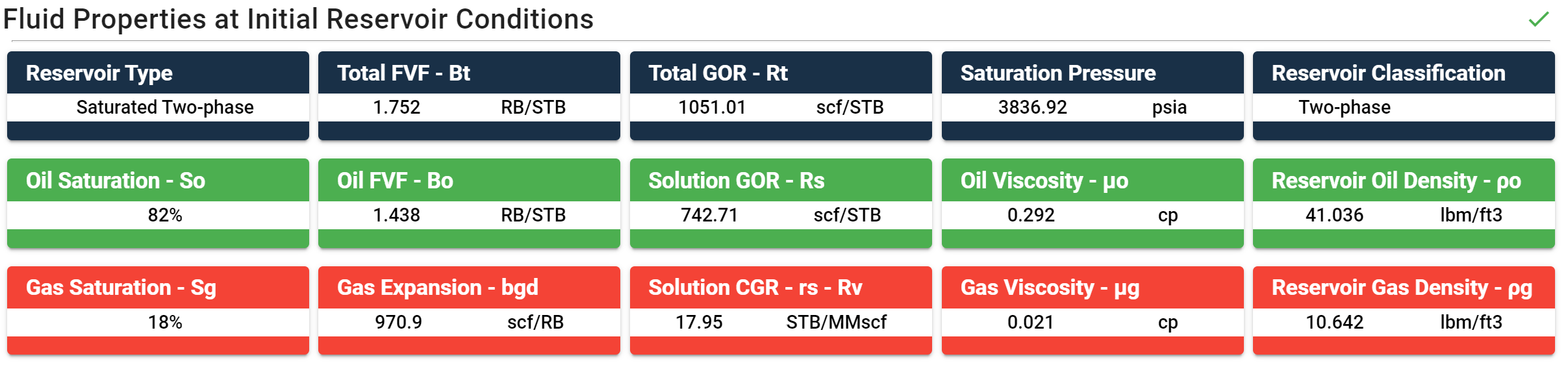
Reservoir Type
Initially, the reservoir can be one of three types:
| Reservoir Type | Saturation Condition |
|---|---|
| Undersaturated oil reservoir | |
| Undersaturated gas reservoir | |
| Saturated two-phase reservoir | and |
Total FVF
Total FVF is defined as:
For an undersaturated oil reservoir (\(S_\mathrm{g} = 0\%\)), this simplifies to \(B_\mathrm{t} = B_\mathrm{o}\). For an undersaturated gas reservoir (\(S_\mathrm{o} = 0\%\)), it simplifies to \(B_\mathrm{t} = \frac{B_\mathrm{gd}}{r_\mathrm{s}}\). For a two-phase saturated case, the total FVF represents a saturation-weighted oil FVF.
Total GOR
Total GOR is defined as:
For an undersaturated oil reservoir (\(S_\mathrm{g} = 0\%\)), this simplifies to \(R_\mathrm{t} = R_\mathrm{s}\). For an undersaturated gas reservoir (\(S_\mathrm{o} = 0\%\)), it simplifies to \(R_\mathrm{t} = \frac{1}{r_\mathrm{s}}\). For a two-phase saturated case, the total GOR represents a saturation-weighted GOR.
Using Total GOR and FVF for In-Place Volume Estimates
Irrespective of reservoir type, total FVF (\(B_\mathrm{t}\)) and total GOR (\(R_\mathrm{t}\)) can be used directly to calculate original oil in place: \(N = \frac{HCPV}{FVF_\mathrm{tot}}\) and original gas in place: \(G = N \cdot R_\mathrm{t}\)
Saturation Pressures
The saturation pressure (bubblepoint or dewpoint) is always the saturation pressure of the fluid definition composition (\(z_{\mathrm{bo}i}\)).
Initial Pressure vs. Saturation Pressure in Saturated Reservoirs
In the case of a saturated two-phase reservoir, the initial reservoir pressure will be lower than the saturation pressure of \(z_{\mathrm{bo}i}\).
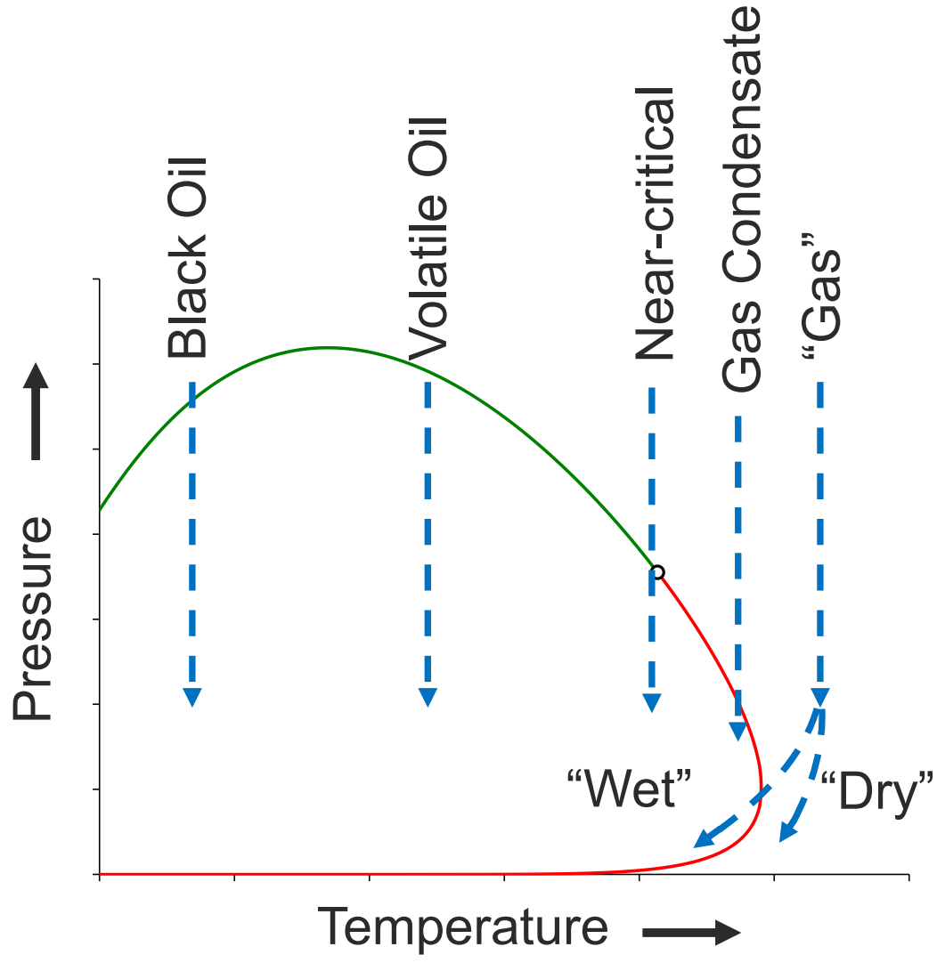
Reservoir Classification
| Fluid Type | C7+ (mol%) | Bo | Bgd/rs (Bgd/Rv) (RB/STB) | Rs | 1/rs (1/Rv) (scf/STB) | Description |
|---|---|---|---|---|
| Black Oil | > 25 | < 1.5 | < 1,000 | - |
| Volatile Oil | 14 - 25 | 1.5 - 2.5 | 1,000 - 3,000 | bubblepoint saturation pressure |
| Near-critical | 11 - 14 | 2.5 - 4 | 3,000 - 4,000 | - |
| Gas Condensate | 1 - 11 | 4 - 50 | 4,000 - 100,000 | Dewpoint saturation pressure |
| Wet Gas | < 1 | > 50 | > 100,000 | No dewpoint at reservoir conditions, but produces liquids at surface |
| Dry Gas | 0 | 0 | ∞ | No dewpoint at reservoir conditions and no liquid production at surface |
| Two-phase | - | - | - | \( S_\mathrm{g} > 0\% \) and \( S_\mathrm{o} > 0\% \) |
Warning
These numbers are rules of thumb and should not be interpreted as absolutes.
Reservoir Density
Reservoir densities are calculated based on black-oil properties as
- Reservoir oil density: \(\rho_\mathrm{o} = \frac{62.4 \gamma_o + 0.0136\gamma_g R_s}{B_o}\)
- Reservoir gas density: \(\rho_\mathrm{g} = \frac{62.4 \gamma_o + 0.0136\gamma_g (1/r_s)}{B_{gd}/r_s}\)
with \(\rho_\mathrm{o}\) and \(\rho_\mathrm{g}\) in lbm/ft³, \(B_o\) and \(B_{gd}/r_s\) in RB/STB, and \(R_s\) and \(1/r_s\) in scf/STB.
Density Calculation Source
The reservoir densities are calculated with the black oil table properties (not from the EOS model).
Modified Black Oil PVT Properties
The Modified Black Oil PVT properties (\(B_o\), \(R_s\), \(\mu_o\), \(B_gd\), \(r_s\), \(\mu_g\)) correspond to the fluid properties for the well at initial reservoir conditions and are extracted from the black oil table for \(p = p_\mathrm{res, init}\).
| Symbol | Property | Description |
|---|---|---|
| Oil FVF | Oil formation volume factor | |
| Solution GOR | Gas dissolved in oil at reservoir conditions | |
| Oil viscosity | Viscosity of the oil phase at initial conditions | |
| Dry gas FVF | Gas formation volume factor at dry gas reference | |
| Solution CGR | Condensate-gas ratio (always included in modified black oil tables) | |
| Gas viscosity | Viscosity of the gas phase at initial conditions |
The black oil tables are "modified black oil tables", which means that the solution CGR (\(r_s\)) is always included in the table. The tables are also extrapolated to a critical point when possible; see here for further details. Read more about black oil PVT here.
3. Export Formats
whitson+ supports several export formats of black oil tables:
- ECLIPSE
- KAPPA
- HARMONY
- CMG IMEX
- RESFRAC
- TNAVIGATOR
- EXCEL
- POWERS
- PROSPER
Custom Export Format Requests
If there is an export format you are missing, send an e-mail to support@whitson.com and we'll implement it for you.
ECLIPSE
The ECL100 BO table created by whitson+ contains one of two combinations:
- PVTO+PVTG: For all fluids that can experience two-phase conditions at the reservoir temperature
- PVDG: For all wet and dry gases that have no saturation pressure at the reservoir temperature.
The combination PVTO \((R_s, B_o, \mu_o)\) and PVTG \((R_v, B_{gd},\mu_g)\) is the most accurate BOPVT formulation for the actual phase behavior, and is referred to as the modified BOPVT formulation. This requires OIL, GAS, DISGAS, and VAPOIL specified in the RUNSPEC section.
Some PVT vendors will provide the combination PVTO+PVDG, which is referred to as the traditional BOPVT formulation (i.e., \(R_v=0.0\) at all pressures / no VAPOIL in model).
The ECL BOT generation includes many of the consistency checks that ECL imposes on the BOT:
-
Negative compressibility checks at 30 equally spaced pressure points from minimum pressure to maximum pressure in the BOT (same table of pressures as ECL). Interpolation and calculation of numerical derivatives are done the same way as ECL.
-
Monotonicity and uniqueness checks for saturated properties: ECL requires \(R_s\) to be monotonic and \(R_v\) to be unique.
-
Monotonicity checks of undersaturated \(B_o\)
-
Physical checks \(\mu_g\leq \mu_o\), \(\rho_g\leq\rho_o\), \(R_s\leq 1/R_v\), \(B_o\leq B_{gd}/R_v\)
All these checks are applied in an attempt to limit the PVT issues / warnings when using the BOT file in ECL100 simulations. To limit issues with initialization and internal extrapolation of the BOT, which can lead to severe runtime issues, we always extrapolate the BOT by the following two steps:
-
Physical Extrapolation: Incipient-phase swelling of composition to calculate saturated properties at higher saturation pressures
-
Artificial Extrapolation: Saturated points are graphically extrapolated up to the initial reservoir pressure + a threshold. This represents the maximum saturation pressure and is by design a critical/convergence pressure where the oil- and gas BOT properties become equal.
KAPPA
Kappa can import Eclipse BO tables. Choose the "import from ECLIPSE" option in Kappa and import the BO table.
Saphir (Pressure Transient Analysis) & Topaze (Rate Transient Analysis)
Step-by-Step: Import black oil table into Topaze(RTA) and Saphir (PTA)
To input the BO tables from whitson+ into Topaze and Saphir, follow these steps:
- Choose the multiphase option
- Pick your reference fluid, either gas or oil
- Check the option to "Define advanced PVT"
- Click on the "Lab Flask" icon to input the black oil table
- From the import options, pick Eclipse and select the file exported from whitson+
- Pick "set the value of GOR / CGR in order to select the closest corresponding under-saturated set of data"
- Input the GOR or CGR (for oil or gas respectively) that you see in the fluid initialization section
- Press OK to close the PVT input window, and then next
- The analytical parameters (formation volume factor and viscosity) are taken from the BO table, and should not be changed. As a QC, you can check that these values are the same as what you get in the fluid initialization section. Go to the next screen.
- Under numerical parameters > Non-linear diffusion > Common functionalities > select "Use real PVT" to ensure that the input black oil table is used in your numerical model (non-linear)
Rubis (Multi Purpose Full Field Numerical Model)
Step-by-Step: Import black oil table into Rubis
To input the BO tables from whitson+ into Rubis, follow these steps:
- Click on the "Lab Flask" icon to input the black oil table
- From the import options, pick Eclipse and select the file exported from whitson+
- When prompted that the "Loaded file contains MBO model" Pick the PVT model that corresponds to the fluid you are importing, either "condensate gas" or "volatile oil". Even if your fluid is not a "volatile oil" or a "condensate gas", you should choose one of these options to ensure that Kappa software takes in the complete modified black oil tables for your analysis
- Pick "set the value of GOR / CGR in order to select the closest corresponding under-saturated set of data"
- Input the GOR or CGR (for oil or gas respectively) that you see in the fluid initialization section
- Under "Reference Parameters" input your initial reservoir pressure and reservoir temperature, the GOR should be the same as you input in step 5
- Press OK to close the PVT input window, and then "Finish"
- Now the PVT model is input and you can proceed to initialize your reservoir model, under
"Properties"> "Initial State".
- Pick "variable type" = composition
- Input the GOR of your fluid, from the fluid initialization section
HARMONY
- We provide an Excel file formatted for a frictionless import into IHS.
- Follow the step-by-step guide below on how to import this table into Harmony.
- For a mass import of black oil tables (30-40 wells) we recommend to set up a database connection and an associated scheduler.
CMG IMEX
The IMEX BO table created by whitson+ is a modified BO table
(it uses the *MODEL *VOLATILE_OIL option, as it is the most flexible option).
In the *INITIAL section (the fluid initialization part of the IMEX file), it is important to define both *PB and *PDEW with the associated
initial saturation pressure. *CON refers to constant compositions (while there are other alternatives that are described well
in the IMEX manual).
*INITIAL
********************************************************************************
** Initial Conditions Section in CMG IMEX                                     **
********************************************************************************
*VERTICAL *BLOCK_CENTER *WATER_OIL_GAS ** Use vertical equilibrium calculation.
*PB *CON    3000          ** bubblepoint pressure
*PDEW *CON    3000          ** dewpoint pressure

*REFDEPTH   8400.           ** Give a reference depth  and
*REFPRES    4800.           ** associated pressure.
*DWOC       20000.           ** Depth to water-oil contact
*DGOC       20000.           ** Depth to gas-oil contact
RESFRAC
The ResFrac BO table created by whitson+ is a modified BO table
(it uses the variable name usemodifiedblackoilmodel to activate this).
There are two ways of importing a BOT in ResFrac
- From frontend: use the "import black oil table from whitson+" option in the Fluid Model Options Tab
-
In simulation deck: copy paste text in the BOT file directly into the text file deck.
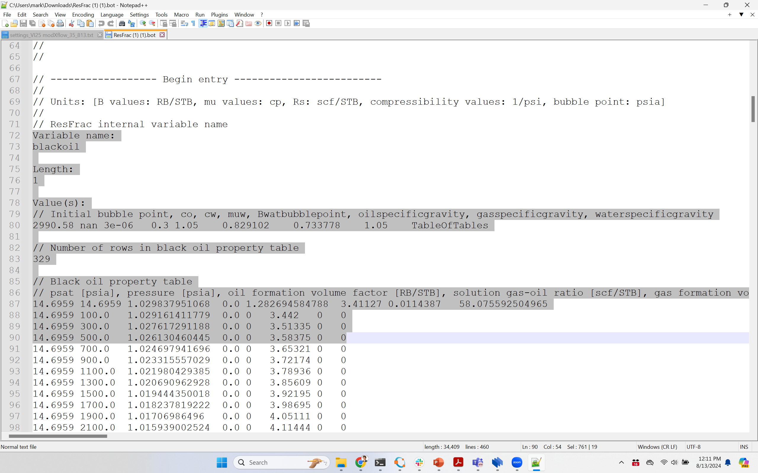
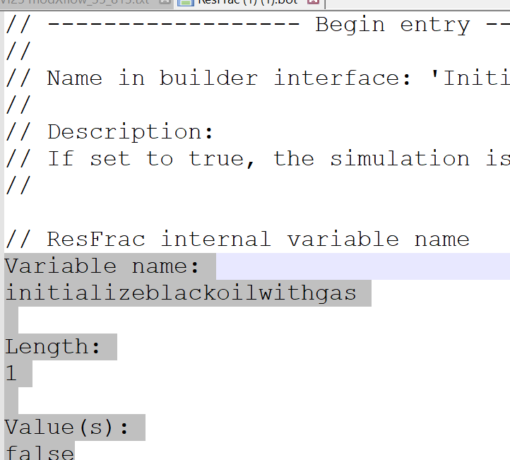
This .bot file has three keywords in it: blackoil, initializeblackoilwithgas, and usemodifiedblackoilmodel.
Open the raw settings file from your simulation:
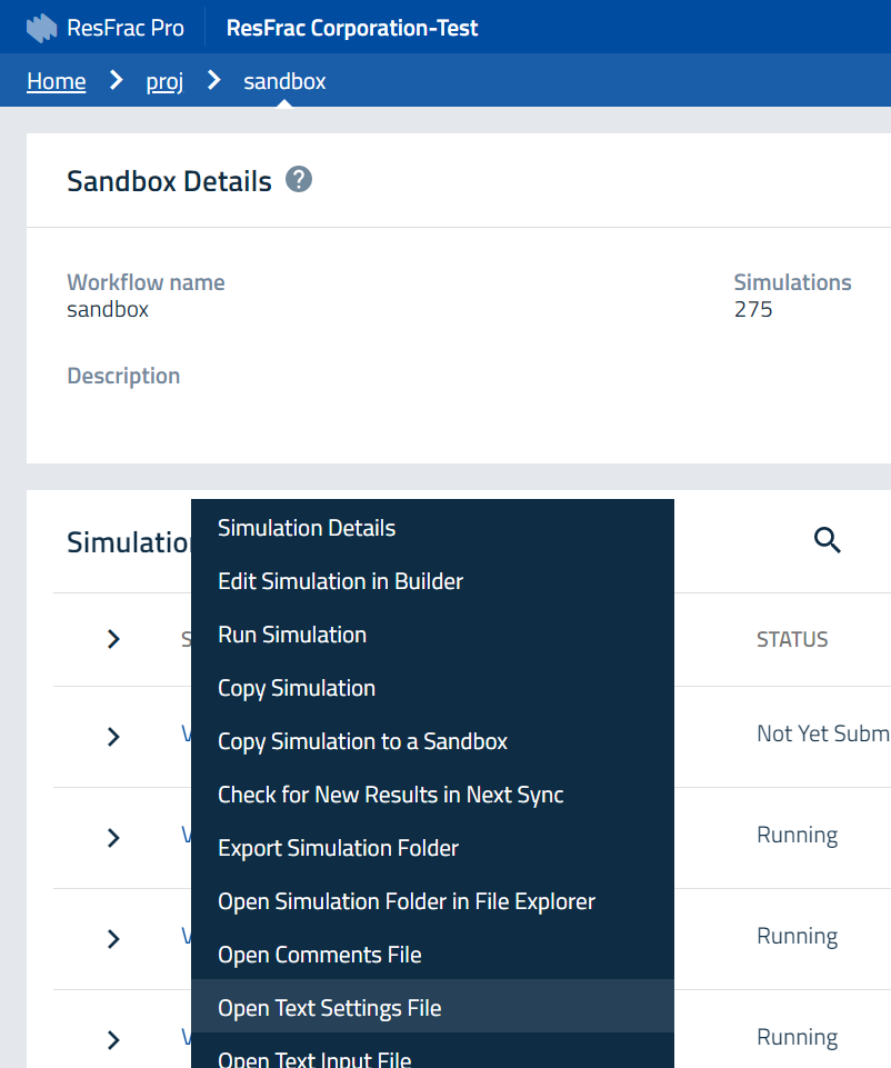
Then find each of the keywords, along with their "length" and "Value(s):" and copy paste it all from the .bot file to the settings file, replacing the values for blackoil, initializeblackoilwithgas, and usemodifiedblackoilmodel that are there now.
TNAVIGATOR
The ECLIPSE BO table created by whitson+ is a modified BO table
(it uses the PVTG keyword to provide \(r_\mathrm{s}\) / \(R_v\) values).
Two sections need to be modified:
TABDIMSKeyword
Modify the TABDIMS section in RUNSPEC using the values for NPPVT
and NRPVT provided in the exported BO table.
For example:
-- !-------------!
-- !             !
-- !   WARNING   !
-- !             !
-- !-------------!
-- TABDIMS should be modified in the RUNSPEC section of your file, to increase the maximum entries in the BO table.
-- Replace TABDIMS in your file by numbers larger or equal (>=) to the ones provided below.
-- XXXX should be kept as currently specified in your TABDIMS keyword.
-- TABDIMS
-- XXXX     XXXX    XXXX     117     XXXX   87  /
-- NTSFUN   NTPVT   NSSFUN   NPPVT   NTFIP   NRPVT
- Water Properties
Modify the water properties in the BO table directly.
-- PVTW Section
-- Default water properties are provided here.
-- These should be changed to appropriate values for your fluid system.
-- Pref (psia)  Bw (rb/STB)  cw (1/psia)  Visco_w (cp)  water viscosibility (1/psia)
PVTW
 14.696   1  3.0E-6  0.5  0  /
EXCEL (whitson)
The Excel export format contains:
- All saturated data (original sample depletion and extrapolation)
- All under-saturated data
- Fluid initialization data (BO properties at initial reservoir pressure)
- Standard BO plots (BO properties for the initial in-situ reservoir fluid)
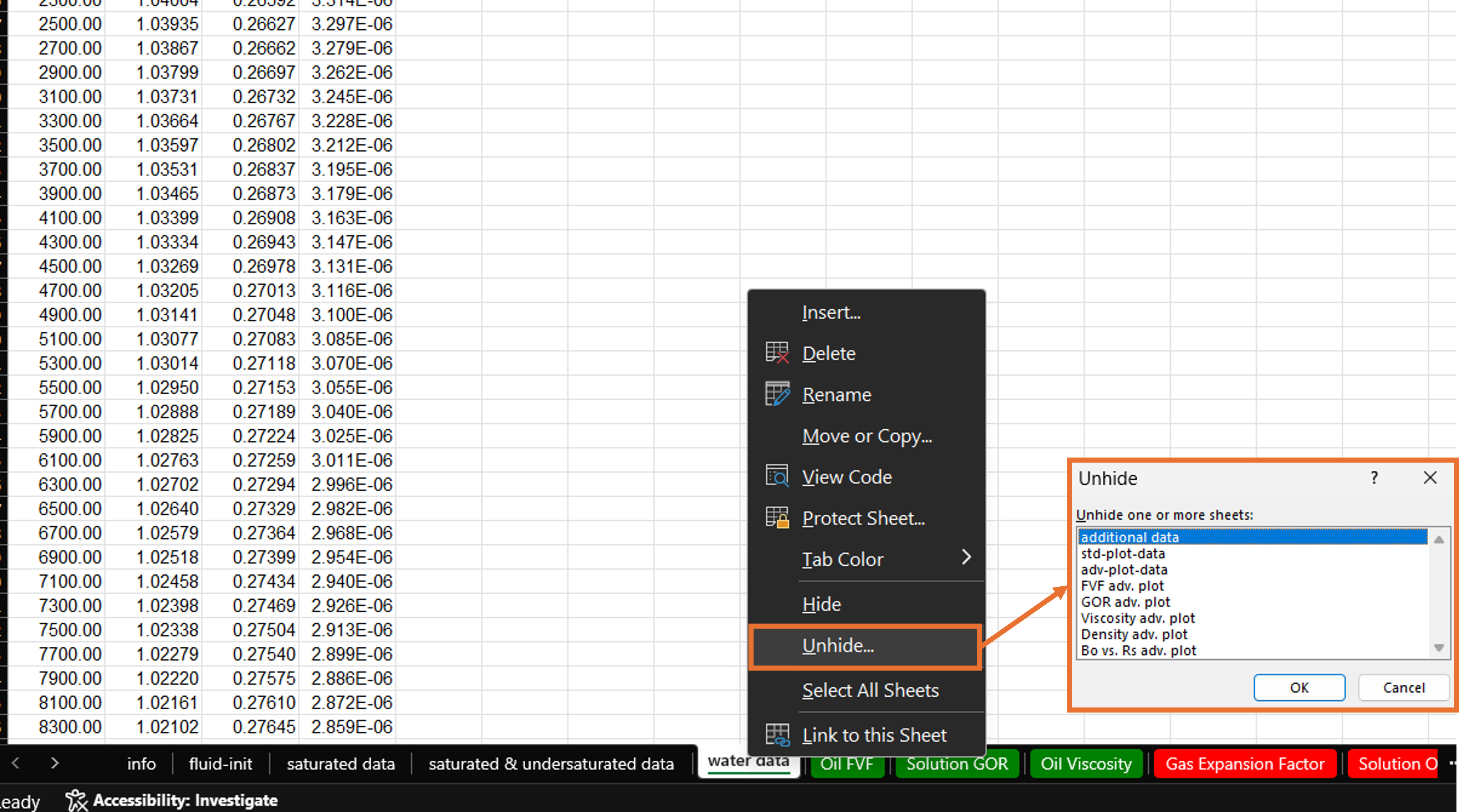
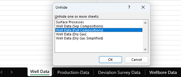
Hidden Sheets
Advanced quality check plots are by default hidden in the excel file, but can be accessed by clicking "Unhide" and picking the relevant plots.
- Advanced BO plots
- Water Data
- Units
POWERS
The POWERS BO table by whitson+ is a modified BO table extrapolated to the critical point if found. It provides the saturated table for both oil and gas. For each saturated pressure in the oil table, the compressibility and viscosibility are calculated. This is used internally in GigaPOWERS and TeraPOWERS to calculate the PVT properties in the undersaturated region.
Compressibility (\(c_{o}\)) is calculated for each saturated point using the undersaturated data predicted by EOS, using the following equation
- \(p_{sat}\): saturation pressure
- \(p_{ref}\): pressure closest to reservoir pressure if pres > psat, else first undersaturated pressure
- \(B_{sat}\): Bo at saturation pressure
- \(B_{ref}\): Bo closest to reservoir pressure if pres > psat, else first undersaturated Bo
Viscosibility (\(c_{\mu_o}\)) is calculated for each saturated point using the undersaturated data predicted by EOS, using the following equation
- \(p_{sat}\): saturation pressure
- \(p_{ref}\): pressure closest to reservoir pressure if pres > psat, else first undersaturated pressure
- \(\mu_{sat}\): Viscosity at saturation pressure
- \(\mu_{ref}\): Viscosity closest to reservoir pressure if pres > psat, else first undersaturated viscosity
PROSPER
The Prosper BO table will require desired reservoir pressures:
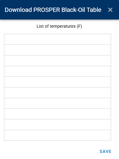
Then it will give properties for each pressure provided, such as saturation pressure, oil FVF, GOR, oil density, etc.
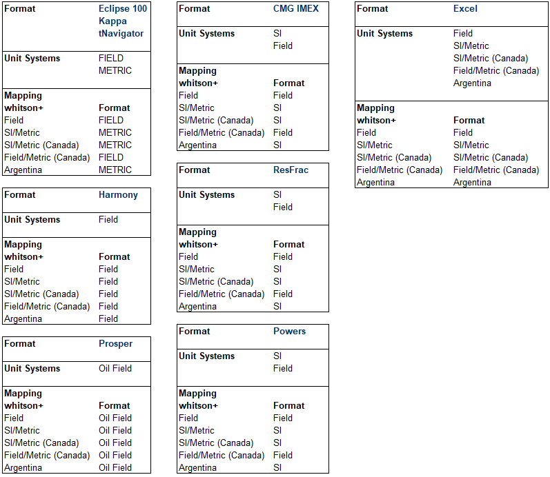
Export Unit System Mapping
This table summarizes which unit system each export format expects, and how whitson+ project unit systems map into those formats during export.
Why this is useful
Use this as a quick QC if your exported file looks like it is in the wrong units.
4. PVT / Fluid Map Workflow
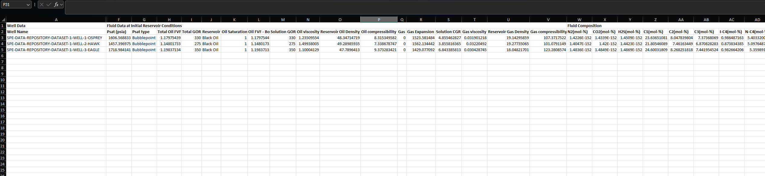
Exporting to well information data automatically generates an Excel file with the data in the phase envelope figure.
To calculate and export PVT properties using the whitson+ EOS for all wells at once:
-
Download the mass upload file: Go to Wells, MASS UPLOAD, WHITSON, and click "DOWNLOAD EXCEL TEMPLATE".
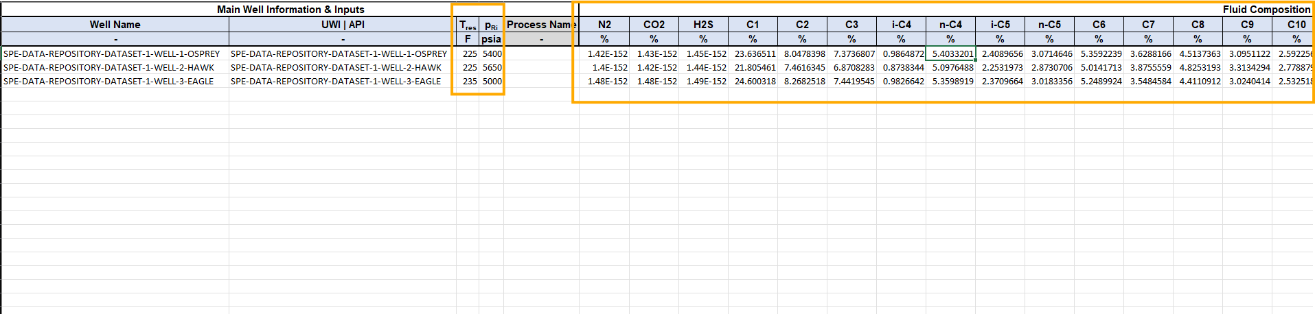
-
Use the sheets that include "Well Data" in the sheet name, and make sure all required fields are populated. Required inputs may include items such as Tres, pRi, and fluid composition, depending on the selected fluid definition method.
Hidden Sheets
Some of the sheets in the Excel template are hidden by default and are dedicated to different fluid definition methods. Unhide the Well Data sheet you need, complete the required fields, and leave the other sheets hidden or unused.
-
Upload the file: Go to Wells, MASS UPLOAD, WHITSON, click "Upload Excel file (.xlsx)", and "SAVE".
-
Bulk Run: Go to Wells, select the wells, click RUN, click "PVT", then click Yes.
-
Bulk Export: Go to Wells, select the wells, click EXPORT, click "Well Information Data", check the boxes for "Well names", "Fluid Data at Initial Reservoir Conditions", and "Fluid Composition", then click EXPORT.
-
An Excel file will be generated with all the PVT properties for the selected wells.
Reservoir Fluid Composition Method
Using the hidden sheet "Well Data (Full Compositions)" to upload wells will set the fluid composition to "Fluid Composition" by default. Using the other Well Data sheets will set the fluid definition method to the corresponding method.
Reservoir Fluid Composition Method
If you enter only the GOR value in the whitson+ mass upload file, the reservoir fluid composition method will be set to GOR. If you provide both GOR and Initial API Gravity, the method will be set to GOR+API.
5. PVT Table Generation: Advanced Topics
All PVT tables provided by whitson+ are modified (i.e. including solution CGR / ), extrapolated BO tables. These tables consist of three parts:
- The depletion of the initial in-situ reservoir fluid
- The extrapolation (eventually to a critical point)
- Average surface densities for oil and gas
Black Oil PVT Table
A black oil table is a two-component PVT model (oil and gas). Three properties are defined for each component:
- Composition ( | ) - surface process dependent
- Formation Volume Factor ( | ) - surface process dependent
- Viscosity ( | ) - surface process independent
The following are assumed to be constant in a black oil table:
- Surface oil and gas densities
- Surface process (#stages, Tsep, psep)
- Reservoir temperature
Required Input
The required input data for generating a modified black oil table is:
- The composition of the initial in-situ reservoir fluid ()
- The reservoir temperature ()
- A surface process () (multi-stage process)
- An Equation of State (EOS) model tuned to the relevant PVT data
Depleted Part of the Table
This part of the table includes mixtures with a saturation pressure ranging from standard pressure to the original saturation pressure of .
A Constant Composition Experiment (CCE) is simulated using . At each stage of the CCE, the equilibrium phases are processed through the surface process and the modified black-oil properties (, , , , , ) are calculated.
Extrapolated Part of the Table
This part of the table includes mixtures with a saturation pressure greater than the original saturation pressure of . Those mixtures are obtained by extrapolating the initial in-situ composition .
Search a Critical Mixture
Definition
A mixture is considered critical if all its K-values ( where and are the gas and oil molar fractions of component , respectively) are equal to 1 at its saturation pressure and reservoir temperature.
The procedure to find a critical mixture is as follows:
- Flash the initial in-situ reservoir composition () at its original saturation pressure. The obtained equilibrium phase compositions are called () and ().
- Re-combine the equilibrium phases using a ratio :
- Calculate the saturation pressure of the resulting composition and its K-values .
- Calculate an RMS error () quantifying the deviation from 1 of the K-values: where is the set of components (e.g. ). Minimize by changing .
Two cases can occur:
- The final mixture satisfies the critical criterion (for all \(i \in \mathcal{C}\), \(K_i = 1\)). In that case, is a critical mixture.
- The final mixture \(z_{\mathrm{c}i}\) does not satisfy the critical criterion. This usually indicates that the saturation calculation blows up at some point; see Case 3 for more details.
Swell Test Check
Finding a critical mixture by extrapolating the original in-situ composition is not sufficient to ensure a consistent extrapolated BO table. We run a swell test on the initial in-situ composition to check if the critical point is admissible. The swell test uses the initial in-situ composition () as a starting point and injects its incipient phase.
Three cases can occur:
Definition: Correct/Wrong Side of the Swell Test
In the following section, we refer to the correct and wrong side of the swell test. Typically, in a swell test, the mixture saturation pressure increases until a maximum value (obtained for a fraction of incipient fluid injected called ). The correct side of the swell test includes all fractions satisfying: The wrong side of the swell test includes fractions satisfying:
Case 1
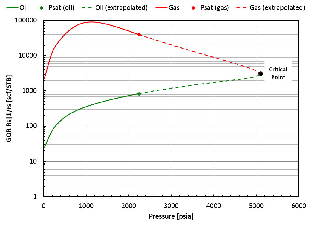
A critical mixture was found using the method presented above, and it is located on the "correct" side of the swell test. See the figure below.
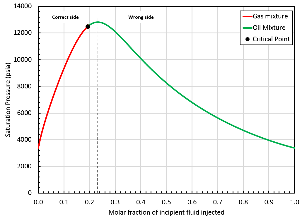
In that case, whitson+ can provide an extrapolated BO table up to the critical mixture (). Such a BO table offers a smooth transition from oil to gas mixtures; see the figure below.
Case 2
A critical mixture was found using the method, but it is located on the "wrong" side of the swell test. See the figure below.
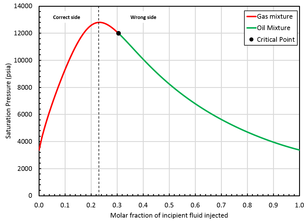
In that case, the BO table will be extrapolated up to the saturation pressure of the found critical mixture (), but by staying on the correct side of the swell test. This is not a critical mixture, so there is a gap between oil and gas properties at the highest pressure in the table; see the figure below.
Case 3
The critical mixture search method failed to find a critical mixture, and the swell test blows up at some point. See the figure below.
Critical Mixture Search Failure and Swell Test Instability
Laboratory examples of swell tests that "blow up" / "do not close" are given in Chapter 8 of the SPE Phase Behavior Monograph by Whitson and Brulé [4].
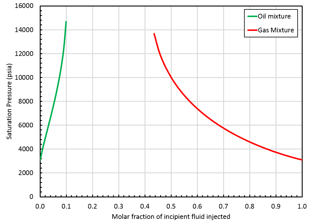
In that case, whitson+ will provide a BO table extrapolated up to the highest finite saturation pressure found on the correct side of the swell test. This saturation pressure is obtained for a mixture that we call . Note that is not a critical mixture; therefore, there is a gap between oil and gas properties at that pressure.
Depletion Experiment for the Extrapolated Part of the Table
A CCE (Constant Composition Expansion) experiment of is simulated from its saturation pressure until the saturation pressure of the initial in-situ reservoir mixture (). At each stage of the CCE, the equilibrium phases are processed through the surface process and the modified black-oil properties (, , , , , ) are calculated.
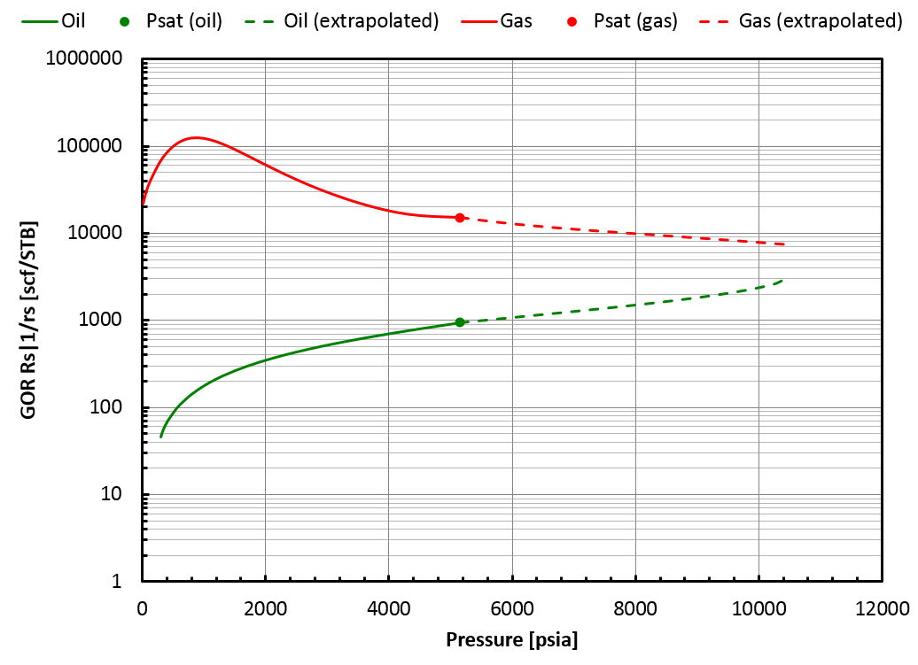
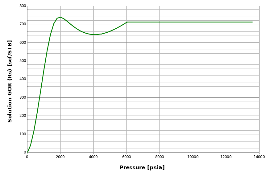
Non-Monotonic Behaviors
A non-monotonic behavior of may occur for lean reservoir fluids (e.g. gas condensates), as seen in the figure below. This is physically explained by the fact that the first droplets of condensate that drop out from the reservoir gas are very heavy and get lighter when pressure decreases, thus increasing .
However, even though this behavior is physically correct, many reservoir simulators do not accept non-monotonic input in the BO tables. whitson+ checks for non-monotonic behaviors when generating BO tables. If such behavior is found, then whitson+ applies a modified procedure for both the depleted part of the table and the extrapolated part.
Depleted Part of the Table (non-monotonic )
whitson+ will run two separate CCE simulations (one for oil, one for gas) with different compositions:
- The BO properties of the gas phase are still obtained by simulating a CCE of .
- The BO properties of the oil phase are obtained by simulating a CCE of the incipient oil phase of (this mixture was previously called ).
Extrapolated Part of the Table (non-monotonic )
Since the depleted part of the BO table uses two fluids, for the gas phase and for the oil phase, whitson+ will perform two separate extrapolations to avoid non-smooth behavior at the junction of the two parts of the BO table:
-
The procedure described here is applied to the gas phase.
-
For the oil phase, the extrapolation is performed by staying on the "wrong" side of the swell test. This ensures a smooth transition of the oil BO properties.
Warning!
Non-monotonic behavior always leads to BO tables that are not entirely closed (meaning that there is a gap between oil and gas properties at the highest pressure)
References
[4] Whitson, C. H., & Brulé, M. R., SPE Phase Behavior Monograph, 2000.
6. Water PVT From Correlations
Water PVT and viscosity can be computed as a function of pressure, temperature, and salinity. The amount of gas in solution in water can also be included as a fourth variable. This section explains how correlations can be used to estimate water density and viscosity, which are relevant for reservoir simulation and pipe-flow calculations. The summary is based on Chapter 9 of Whitson and Brulé\({^3}\).
Water Salinity
The salinity of water represents the amount of "total dissolved solids" (TDS) in the water, usually consisting mainly of NaCl. The salinity can range from 0 (fresh water) to \(\approx 300{,}000\) ppm (upper limit is temperature dependent). Seawater has a salinity of about 35,000 ppm. Salinity can be expressed in different quantities: weight fraction, \(w_s\); mole fraction, \(x_s\); molality, \(c_{sw}\); weight concentration in parts per million, \(C_{sw}\); and volume concentration in parts per million, \(C_{sv}\).
The limiting concentration for NaCl brine is [3]
with temperature \(T\) in Celsius.
Water Salinity: Definitions, Limits, and Input Format in whitson+
The input for water salinity in whitson+ is weight concentration \(C_{sw}\) (ppm = mg TDS/kg salt water = \(10^6m_s/(m_s+m_w^0)\)), which is converted internally to a weight fraction \(w_s=10^{-6}C_{sw}\) and molality \(c_{sw}=17.1C_{sw}/(10^6-C_{sw})\) used in computations.
Water Density
The mass density of water at a specified pressure, temperature, and salinity is calculated using a water formation volume factor (FVF) through the relationship: where the water FVF is calculated in a two-step procedure:
- At standard pressure and the specified temperature and salinity, compute the water FVF, \(B_{w}^0(T,w_s)\).
- At pressure, temperature, and salinity, compute the water FVF, \(B_{w}(p,T,w_s)\), by correcting \(B_{w}^0(T,w_s)\) with a correction factor \(C=f(p,T,w_s)\).
Surface Water Density
The water density at standard conditions \(\rho_{\bar{w}}^0\) is computed by the correlation:
Water FVF
The water FVF at standard pressure and the specified temperature and salinity \((B_w^0)\) is calculated by the following correlation: where \(\rho_w^0 = A_0+A_1w_s+A_2w_s^2\), with with temperature, \(T\), in K.
The water FVF at pressure, temperature, and salinity is calculated by the following correlation: where \(p_{sc}\) is standard pressure, and with pressure, \(p\), in psia, and temperature, \(T\), in °F.
Water Compressibility
The water compressibility can be derived from the water FVF by the definition of compressibility:
Water Viscosity
Viscosity
The water viscosity is calculated by the following correlation:
where
with
and
The coefficients \(a_{1i}\), \(a_{2i}\), and \(a_{3i}\) are: where viscosity, \(\mu\), is in cp, temperature, \(T\), is in °C, and pressure, \(p\), is in MPa.
Viscosibility
The reservoir simulators Eclipse 100 and OPM Flow compute the water viscosity as a function of pressure through the use of a so-called "viscosibility" defined as:
Assuming that the viscosibility is constant, the viscosity can be expressed as an exponential function of pressure by
where \(p_0\) is the reference pressure at which a corresponding water viscosity \(\mu_w(p_{0})\) is provided together with the viscosibility.
For the water-viscosity expression above, the water viscosibility is expressed by
7. Water PVT From EOS Model
Water properties such as FVF, gas-water ratio (GWR), density, and compressibility are determined using an EOS model.
Required Input
The required input data for generating water properties are:
- the composition of the initial in-situ reservoir fluid (\(z_{\mathrm{bo}i}\))
- the reservoir temperature (\(T_{\mathrm{res}}\))
- brine salinity (\(c_{sw}\))
- an Equation of State (EOS) model tuned to the relevant PVT data (not including water)
Procedure
EOS Model Tuning
Two EOS models are developed, one for the aqueous phase and another for the non-aqueous phase. Søreide-Whitson\({^1}\) and Yan-Huang-Stenby\({^2}\) provide the equations to calculate binary interaction parameters (BIPs) for both phases (aqueous and non-aqueous) for the Peng-Robinson EOS model. These equations are provided in the tables below and are used as initial values in the EOS regression.
Aqueous phase BIPs for PR EOS model used for a water/hydrocarbon system.
| Component | Equation |
|---|---|
|
|
|
|
|
|
Non-aqueous phase BIPs for PR EOS model used for a water/hydrocarbon system.
| Component | Equation/Value |
|---|---|
The modified \(\alpha\)-term in the EOS constant \(a\) for the brine component is calculated as a function of water reduced temperature and brine salinity using the following equation:
-
Brine Density:
Brine density at each pressure is calculated using the Rowe-Chou correlation. Brine salinity (\(c_{sw}\)) and reservoir temperature (\(T_{\mathrm{res}}\)) are used as inputs to this correlation. Then the aqueous EOS model is tuned to match the brine densities by regressing on the critical properties of water. -
Brine Viscosity:
Brine viscosity at each pressure is calculated using the Kestin correlation. Brine salinity (\(c_{sw}\)) and reservoir temperature (\(T_{\mathrm{res}}\)) are used as inputs to this correlation. The third (P3) and fourth (P4) LBC correlation parameters are used to match the aqueous EOS model viscosities to those predicted by the Kestin correlation.
Because the water critical properties of the aqueous EOS model are modified in the steps above to match brine density and brine viscosity, the modified aqueous EOS model is tuned to match the saturation pressure determined from the original aqueous EOS model (with BIPs from the tables presented above).
Calculating Water Properties
After the EOS model is tuned to the brine density and viscosity data, the water properties are calculated as follows:
- Flash a mixture of water (50 mol-%) and the \(C_{4-}\) fraction of the initial in-situ reservoir fluid (\(z_{\mathrm{bo}i}\)) (50 mol-%) at reservoir temperature (\(T_{\mathrm{res}}\)) and the desired pressure using the modified aqueous EOS model.
- Equilibrium liquid and gas from step 1 are brought to \(60^\circ\mathrm{F}\) and 14.7 psia. Then \(B_w\), \(R_{sw}\), \(\rho_w\), and \(\mu_w\) are calculated for the aqueous phase.
- Steps 1 and 2 are repeated using the non-aqueous EOS model to determine \(R_{vw}\) and \(B_{gw}\).
- Saturated \(c_w\) is calculated using the equation below:
where \(R_{sw}'\) and \(B_w'\) are derivatives of \(R_{sw}\) and \(B_w\) for a decreasing pressure change in the saturated state.
- Undersaturated \(c_w\) is calculated from the same equation, where \(R_{sw}' = 0\) and \(B_w'\) is calculated for an increasing pressure change in the undersaturated state:
References
[1] Søreide, I., and Whitson, C. H.: "Peng-Robinson Predictions for Hydrocarbons,
CO2, N2 and H2S With Pure Water and NaCl-Brines," Fluid Phase
Equilibria (1992)
[2] Yan, W., Huang, S., and Stenby, E. H., "Measurement and modeling of CO2 solubility in NaCl brine and CO2-saturated NaCl brine density," International Journal of Greenhouse Gas Control, Volume 5, Issue 6, 2011, Pages 1460-1477, ISSN 1750-5836
[3] Whitson, C. H., and Brulé, M.: "Phase Behavior", SPE Monograph Series vol. 20, ISBN: 978-1-55563-087-4