Auto-Forecast
This module performs a DCA autofit on all streams (oil, gas, and water) for selected wells in a given project. You can have multiple versions of these DCA autoforecasts (for different wells or different ranges of autofit parameters) within a project.
How does the autofit algorithm work?
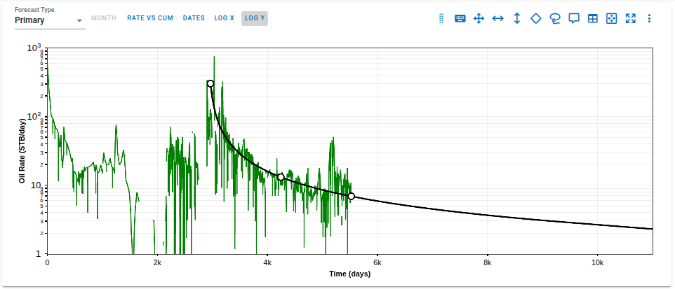
The autofit algorithm finds the timestep with the maximum production data and performs a single-segment or multi-segment best fit from that timestep through the rest of the historical period.
Here's how to create a new autoforecast case:
- Click Auto-Forecast in the navigation panel.
- TIn the upper-right corner, click ADD AUTO-FORECAST.
- Provide a name and select all the wells by clicking the check box at the top of the well list (left of Well Name).
- Click SAVE in the lower-right corner.
You can store multiple auto-forecasts per project
This main autoforecast page gives you an overview of the created auto-forecasts, when they were created, who created them, and what wells went into creating them.
After the autoforecast is created, there are two main steps: 1. Initialize and 2. Autofit.

1. Initialize
This is where Auto-Forecast is initialized by defining fit ranges and other relevant assumptions before running the autofit.
Auto-Forecast settings can be saved within a case:
- Each case can be set to Private or Company-wide.
- Cases can be saved, edited, and updated after creation.
- Saved templates can be reused to update existing setting or create new cases.
- Click Save Name, then provide a name to save the selected settings as a case.
- Once a case is saved, Save Name becomes disabled, indicating no changes have been made since the last save.
- If Save Name is enabled, it indicates there are unsaved changes in the selected case.
- When opening Auto-Forecast Initialize, whitson+ will load the settings last used for autofitting.
1.1. Settings
- b-factor switch: dictates what should happen if the b-factor min or max is the converged solution during the autofit.
When the switch is ON: If the best-fit solution hits the upper or lower b-factor bound, a best-fit is performed using the default b-factor instead.
When the switch is OFF: If the best fit solution hits the upper or lower b-factor bound, that value is used.
- Overwrite: Checking this box allows the Autofit function to update manually fitted wells according to the parameters in the "Initialize" section. If left unchecked, manually fitted wells will not be overwritten.
- Plot Custom Settings: Checking this box provides the option to customize the primary and secondary plots for the fit of each well. As shown below, any parameters selected will be applied to all wells.
- Autofit Decline Type: You can use the Autofit Type dropdown to select between the Arps single-segment decline or the 2-segment Modified Arps decline.
1.2. Bounds
- Autofit ranges:
Default: The starting point for autofit - \(q_i\) is the initial production ratio; b is the rate exponent, or the b-factor, and \(a_i\) is the nominal decline rate.
Min: lower bounds of best-fit solution for \(q_i\), b and \(a_i\).
Max: upper bound of best-fit solution for \(q_i\), b and \(a_i\).
What is the initial production ratio?
This is the ratio between the \(q_i\) that the DCA uses and the maximum production rate found in the production dataset for the well. For example, if you have a given well where the maximum oil production in history is 1000 STB/d, having an initial production ratio between 0.8 and 1.2 means we are allowing the initial rate in DCA to be between 800 STB/d and 1200 STB/d. It is basically a generic way to specify the range for \(q_i\), for a large number of wells, and all the different phases (oil, gas, and water) in one go.
- Streams: It is possible to customize the bounds for each stream (oil, gas, or water). By checking this box, you can select different forecast types, autofit types, rate exponents, peak rates, etc., for each stream.
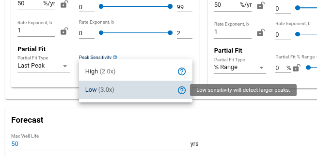
- Partial Data Fitting: This function allows for partial fitting of DCA segments. Checking this box prompts you to input the partial fit type and range.
Note: Last Peak (Partial Fit Type) This option helps fit the data corresponding to re-fracs. It fits the data starting from the last flagged period of elevated rates.
An elevated rate is defined as a rate which is higher than the last 12-month rolling median in production rate times the peak sensitivity. Peak sensitivity can be low (3x) or high (2x). Choosing low sensitivity option will detect large peaks in production and high sensitivity option will detect smaller peaks.
Flagged period is a period with 15+ consecutive days of elevated rates.
- Fit Data Range: Allows you to define optional minimum and maximum limits for each forecast type and stream used in the autofit process. These limits can be specified independently for each stream.
When enabled, the autofit will only consider data points whose rate or ratio values fall within the specified range. Any data points outside the defined limits are excluded from the fit.
Both the minimum and maximum values are optional. You may specify:
- Both a minimum and maximum value
- Only a minimum value
- Only a maximum value
- Neither value
If no minimum value is provided, the minimum is assumed to be 0. If no maximum value is provided, all values above the minimum are included in the fit.
-
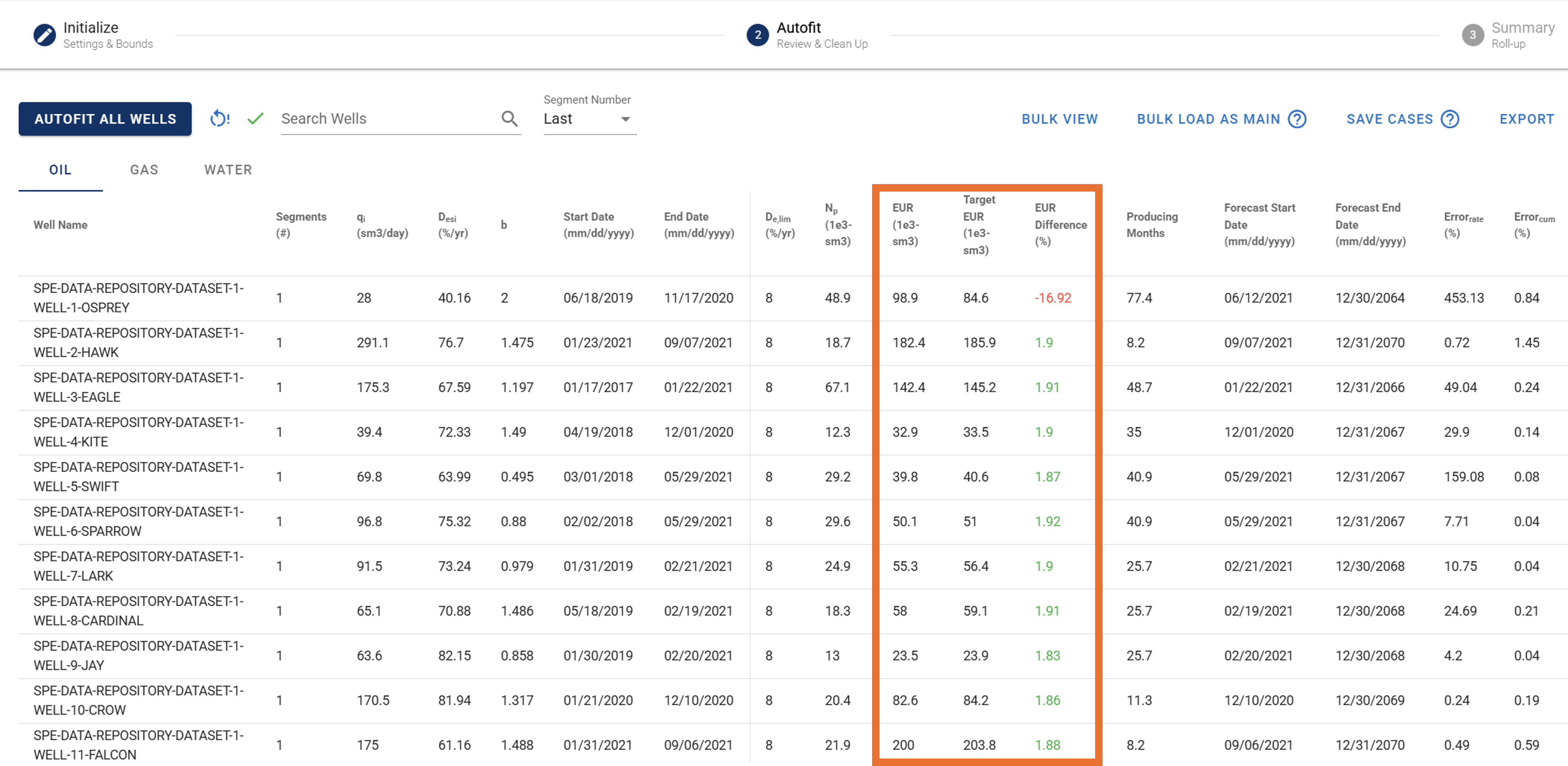
Match EUR: In the standard DCA autofit, the software adjusts qi, Di, and b to minimize the weighted least squares difference between the modeled rates and the historical production. The fit is driven entirely by rate residuals within the specified history range, subject to parameter bounds and any decline limits. The resulting EUR is simply the outcome of the best rate match combined with the forecast assumptions such as limiting decline, cutoff rate, and max well life.
With Match EUR enabled, the model must also satisfy a recoverable volume constraint based on a user-defined EUR tolerance. The tolerance is applied around the target EUR to create an acceptable range. For example, if the target EUR for a well is 100 MSTB and the tolerance is 2 percent, the acceptable range becomes 98 to 102 MSTB. After an initial rate-based fit, the parameters are refined so that the EUR, defined as historical production plus forecast under the specified decline limits, cutoff rate, and well life, falls within this tolerance range. The optimizer prioritizes rate matching while the EUR remains inside the acceptable window, but applies a strong penalty if it falls outside, effectively enforcing the EUR constraint while preserving as much of the history match as possible.
GREEN indicates that the autofitted EUR falls within the specified tolerance range around the target EUR.
RED indicates that the solution could not achieve an EUR within the defined tolerance. In this case, the parameter bounds may be too restrictive, and adjustments to inputs such as b-factor or Di limits may be required to allow a feasible match.
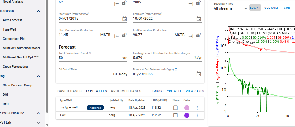
1.3. Forecast
- Total Production Period: Sum of historical time and forecasted time.
- Oil Cut-off Rate: The rate at which to stop the forecast.
- Limiting Effective Decline Rate: Specifies when the hyperbolic decline curve transitions into an exponential decline curve at a specified limiting effective decline rate.
2. Autofit
This section provides an overview of the autofit results. In this view you can filter and manually update the individual fits.
2.1. Autofit all wells
Click "Autofit All Wells" in the upper-left corner to best-fit all the wells in a given project.
2.2. What does Error (%) represent?
whitson+ facilitates regression on parameters to minimize the sum of the squared weighted residuals in the context of observed data and corresponding predictions. The objective function is defined as:
Here, represents the RMS residual error between observed measurement and its corresponding prediction, while is the user-assigned weighting factor for that residual. Ideally, these weighting factors should be inversely proportional to the standard deviations of the residuals. Minimizing provides the maximum likelihood estimate of the model parameters, assuming the residuals are independent and normally distributed.
The default weighting factors are 1. The reported value is the root-mean-square (RMS) residual error () defined as:
This metric is related to but is easier to interpret.
The residuals are calculated as relative percentages using the following formula:
where is the historical production value, is the DCA value, and is the reference value for observation .
For more details on the error calculation, refer to the Error section of the DCA documentation here.
2.3. Sort, Filter and Change Streams.
- Sort: Click the parameter header to sort the well list by that parameter.
- Search: Use the search bar to search for a specific well.
- Change stream: Click OIL | GAS | WATER tabs to switch between the streams.
2.4. Manually Edit
You can manually check and adjust each fit by clicking the row in the table.
- Click the row. A window showing the single-well DCA fit will appear.
- Navigate to the next well with the right arrow (→) and the previous well with the left arrow (←) on your keyboard.
What does the DCA b-factor represent?
DCA fits can be tied to physical parameters as long as the fit is done while the flowing bottomhole pressure is constant (or about constant). The b-factor represents recovery efficiency. A low b-factor indicates a low recovery efficiency. A high b-factor indicates a high recovery efficiency.
2.4.1. Adjusting the autoforecast fit on a well
- Values can be manually entered.
- The fit can also be graphically edited.
- See .gif above (it is just for example purposes).
2.5. Save Fit
Click "Autofit All Wells" in the upper-left corner to save all autofits (for all streams). These forecasts can be appended to the historical data in the Type Well Feature.
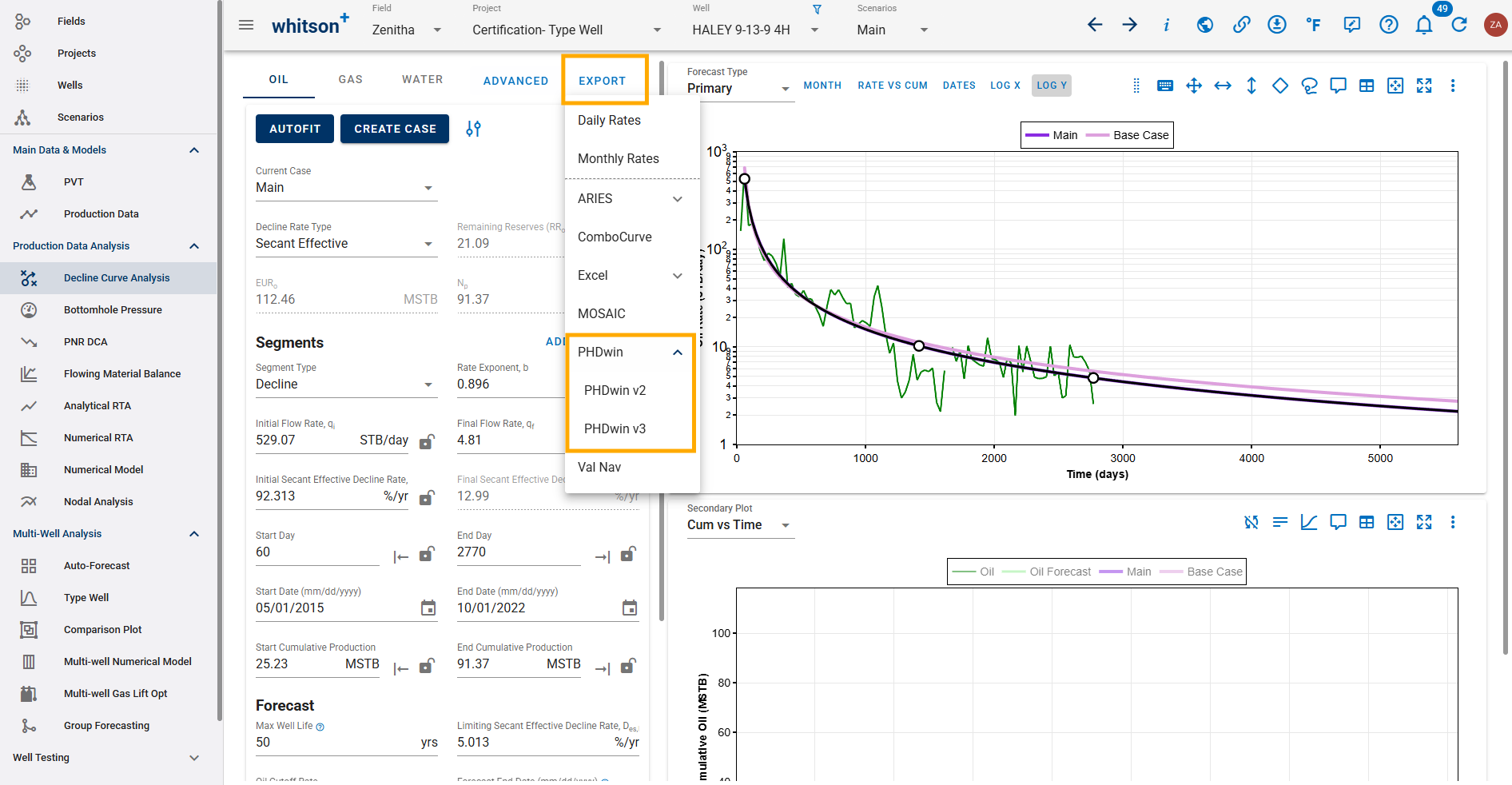
2.6. Export
Click EXPORT in the upper-right corner to export to third-party software (for all streams). whitson+ supports the following for both Auto-Forecast and Forecast Manager:
- Aries
- Excel
- MOSAIC
- PHDwin
- PowerPoint
- Val Nav
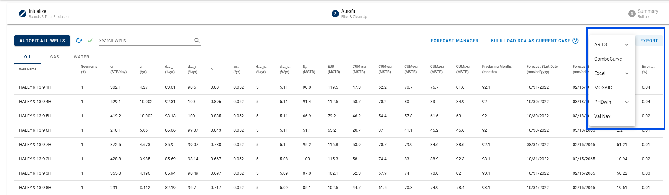
2.6.1. ARIES
You can use this option to export all well declines to ARIES in a single step. Typically, select Export → ARIES → End of Prod. When you click ARIES, the ARIES Export Settings window opens, allowing you to configure both general export options and ARIES-specific settings before exporting the forecasts.
In the Segment Units section, you can choose the production rate units for the forecast, including per day, per month, or per year. You can also select the Time Duration Units, which determine how forecast durations are measured (for example, days, months, or years).
Next, select the Forecast Start Point, which determines where the forecast begins. The available options are First Segment Date, Last Production Date, Custom, and Custom Attribute Date.
Finally, specify the Ending Condition for the forecast. You can end the forecast based on an Ending Rate, which represents a specified production limit (for example, a standard volume per day), or by Time Duration, which defines the total length of the forecast phase.
After configuring the desired settings, proceed with the export as shown in the GIF below.
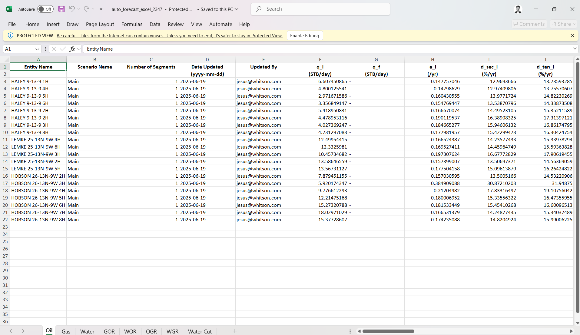
2.6.2. Excel
This option allows you to bulk export all well declines into an Excel file. A typical workflow is: Export → Excel → "End of Prod", then select an Entity Name from the dropdown menu, as shown in the GIF below:
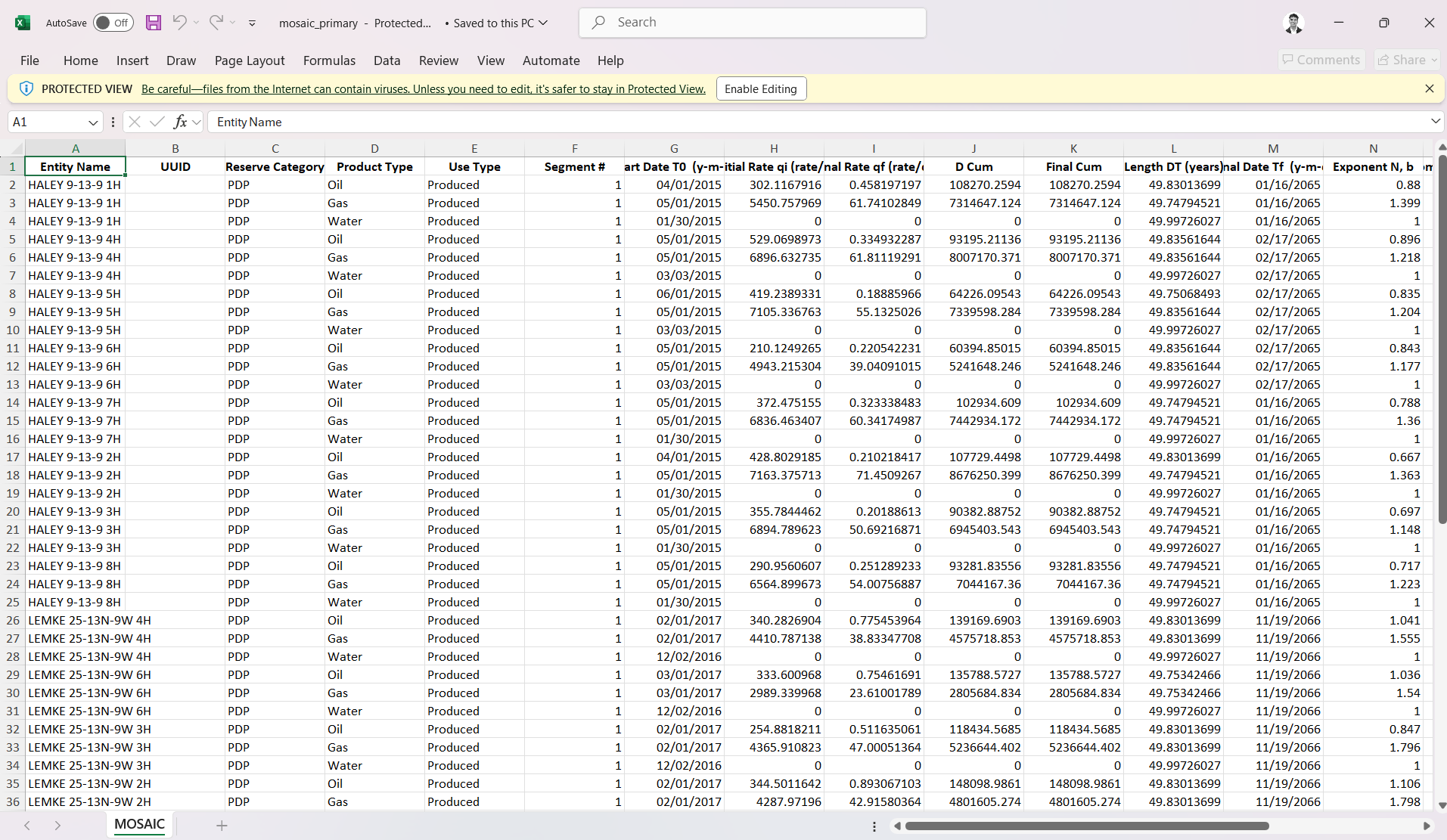
2.6.3. MOSAIC
You can use this option to bulk export all well declines in a MOSAIC-friendly format. This requires selecting an Entity Name from the dropdown menu as shown in the GIF below:
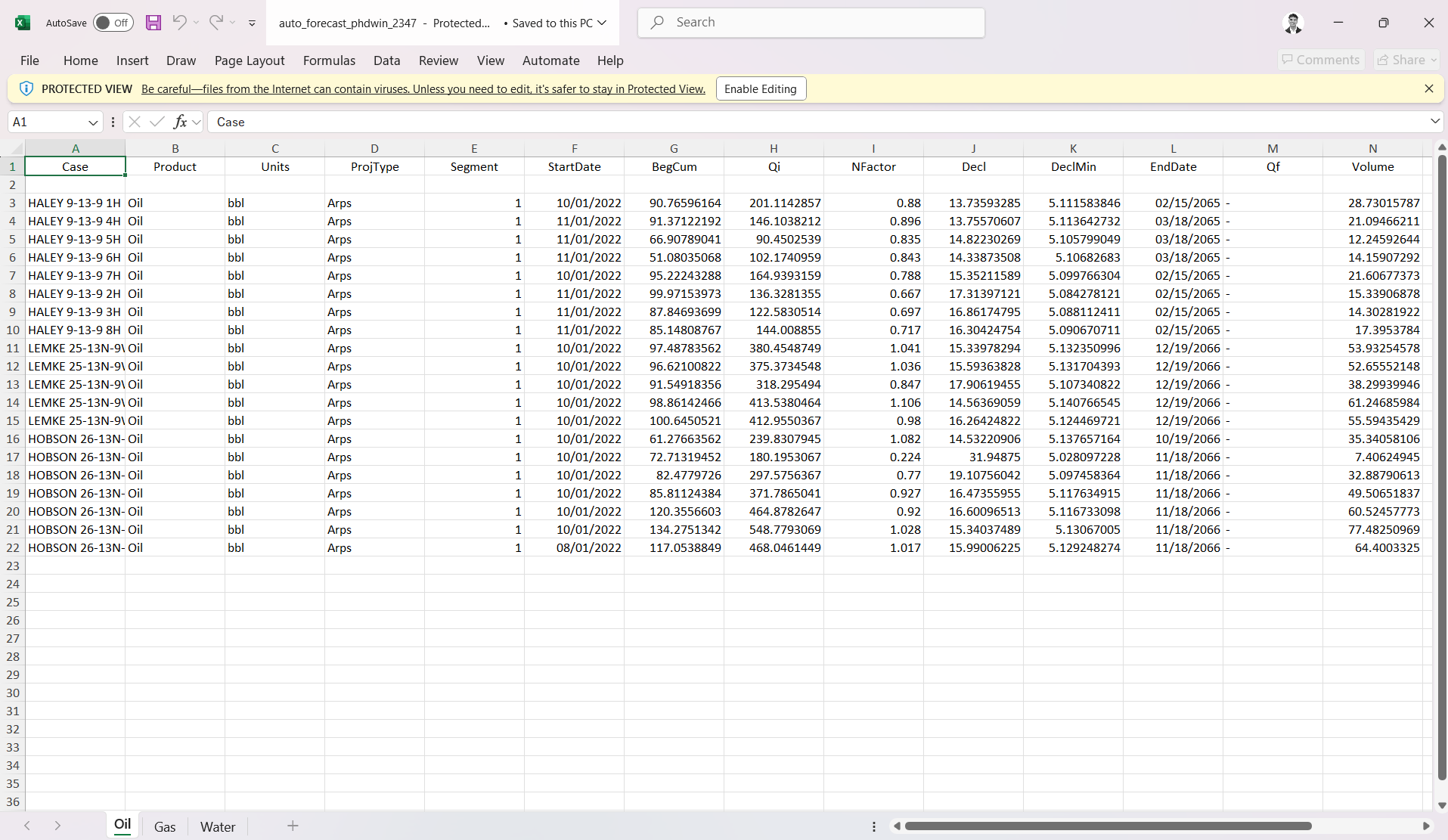
2.6.4. PHDwin
This option allows you to bulk export all well declines into an PHDwin-friendly file. A typical workflow is: Export → Excel → "End of Prod", then select an Entity Name from the dropdown menu, as shown in the GIF below:

2.6.5. PowerPoint
The Export to PowerPoint feature allows you to generate presentation-ready slides containing all well declines. Three export layouts are available, each designed for a different purpose.
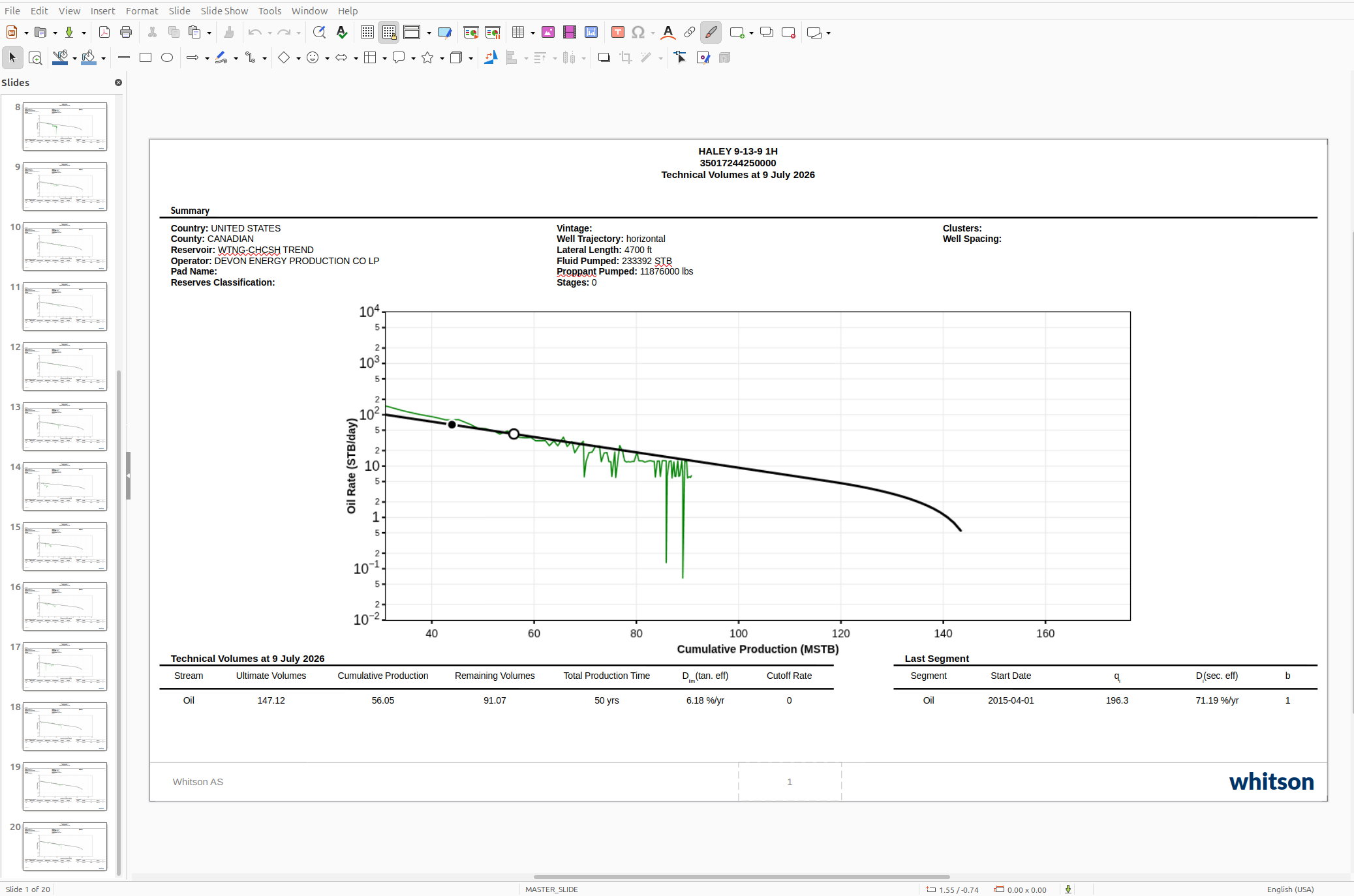
2.6.5.1. Individual Streams
The Individual Streams option exports each selected production stream (Oil, Gas, or Water) on a separate slide. This layout is useful when each stream needs to be presented individually with detailed forecast information. The following options can be customized before exporting:
Select the production streams to include. Use the current DCA zoom. Choose the well title information (e.g., Well Name, UWI, External ID). Select the summary information to display on the slide, such as location, reservoir, completion, reserves classification, fluid pumped, stages, clusters, and other available well attributes. Each selected stream is exported with its corresponding DCA forecast plot and summary tables.

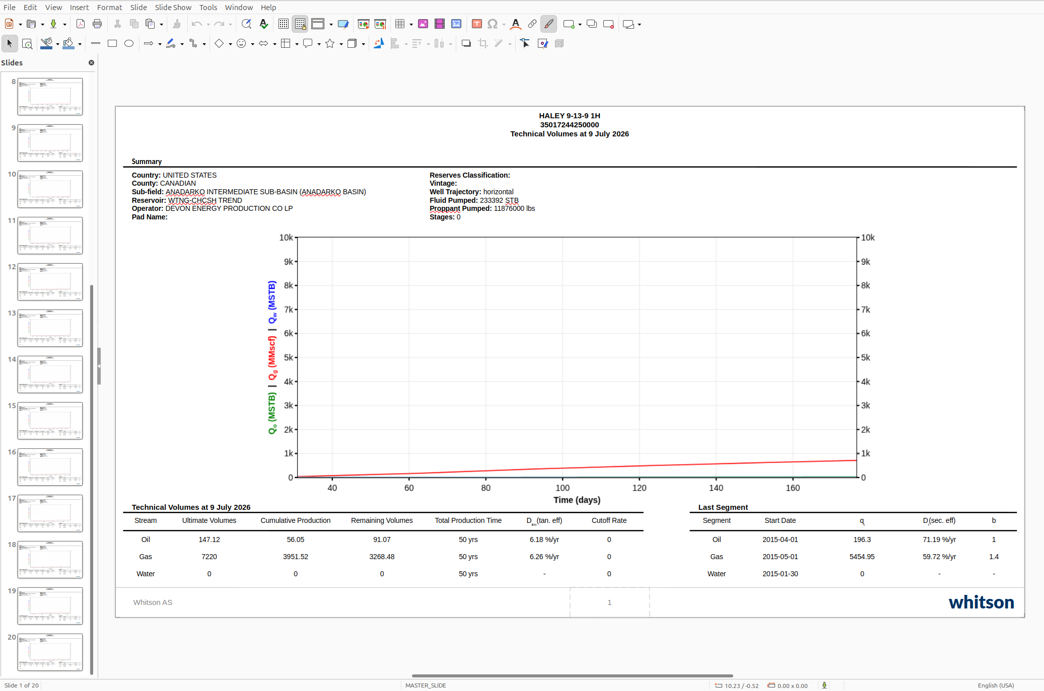
2.6.5.2. All Streams
The All Streams option exports all production streams on a single DCA forecast plot, allowing the Oil, Gas, and Water forecasts to be viewed together on one slide. The same customization options available for Individual Streams are also available here, including:
Using the current DCA zoom. Selecting the title information. Selecting the summary information displayed on the slide.
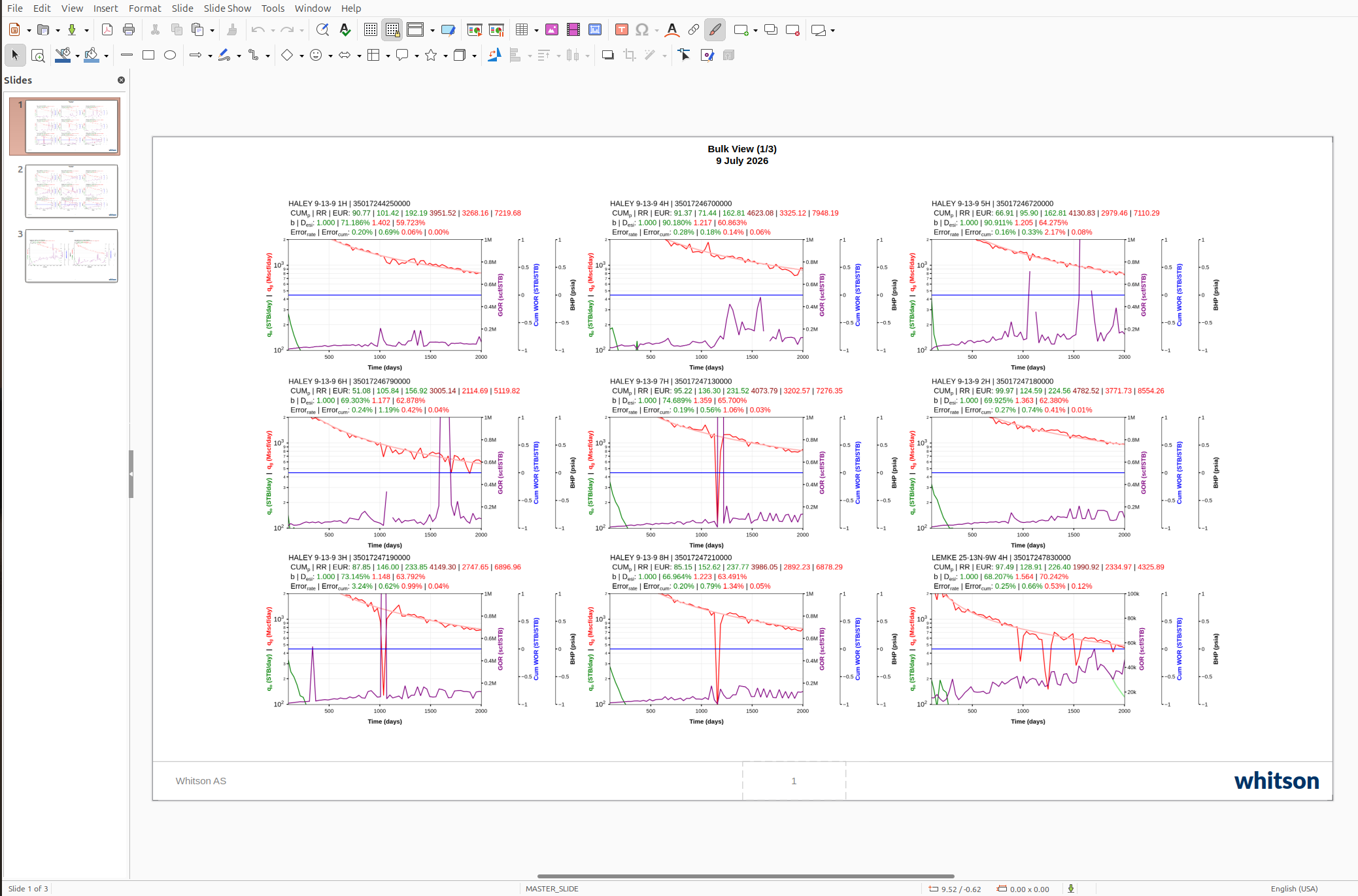
2.6.5.3. Bulk View
The Bulk View option exports the DCA forecast plots for multiple wells on a single slide, making it easy to compare forecast performance across wells. The exported plots can be customized by selecting:
Grid dimensions (number of wells displayed per slide). X-axis settings: Axis basis Time resolution Minimum and maximum values
Y-axis limits. Primary phases to display (Oil Rate, Gas Rate, Water Rate, cumulative production). Ratios, including GOR, WOR, WGR, OGR, and cumulative ratios. Supplemental data such as BHP, line pressure, tubing pressure, casing pressure, choke size, and gas lift.
2.6.6. Val Nav
You can use this option to bulk export all well declines in a Val Nav-friendly format. This requires selecting an Entity Name and a Streams type from the dropdown menu as shown in the GIF below:
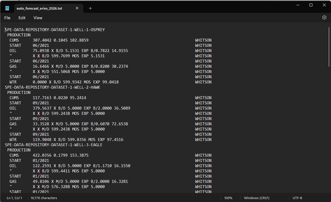
Here are some examples of what export files from whitson+ would look like:
-
Val Nav Decline Import Template.xlsx
Import Notes Regarding Decline Template:
- Only the columns highlighted in green are required for every record.
- Header names must match the expected field names exactly.
- In each header cell, note the expected units of that field.
- Every product decline segment must include a start date, Qi, and three Arps parameters to be considered valid.
- For the first segment, both the start date and Qi are required.
- For the second and later segments, if the start date and Qi are left blank, they will automatically link to the previous segment’s end date and Qf.
- For the second and later segments, you can set Di Linked = True to link Di to the Df of the previous segment.
- All segments within the same product decline must be grouped together and sorted in ascending order by segment index (earliest segment first).
- All product declines within the same entity must also be grouped together, though the order of those grouped declines does not matter.
- Decline types for Di and Df (
nominal,effective tangent, oreffective secant) are interpreted according to the user’s active decline-type setting in their user options. - Slope type can be left blank if ratio declines are not being imported.
-
Val Nav Forecast Constants Import Template.xlsx
Import Notes Regarding Forecast Constants Template:
- Only the columns highlighted in green are required for every record.
- Column headers must match exactly as written.
- The second row defines the unit system and available options, so it must also match exactly.
To import into Val Nav, use Spreadsheet Import in Val Nav to load decline or forecast constant data from the whitson+ export template.
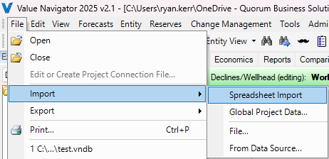
- Go to File > Import > Spreadsheet Import.
- Select the spreadsheet you want to import.
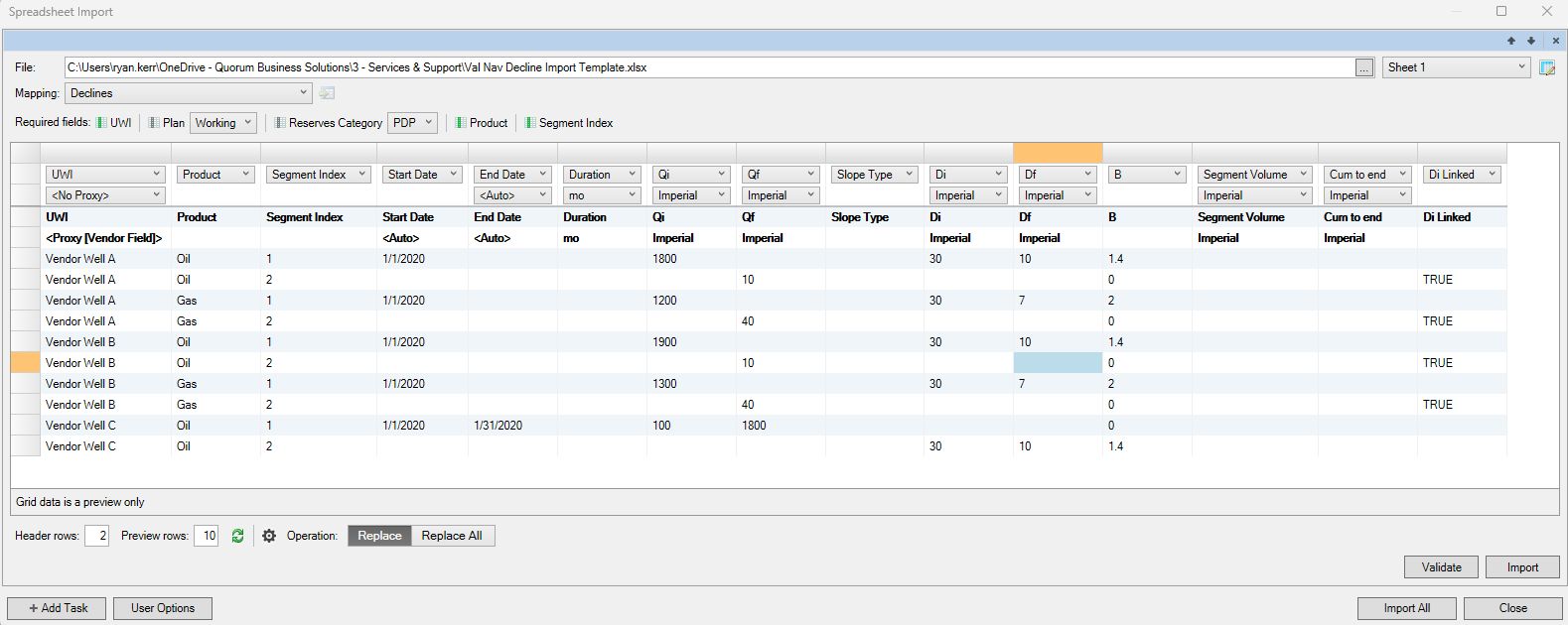
- In the import dialog, set Mapping to either Declines or Forecast Constants, depending on what you are importing.
- Choose the correct forecast destination, such as the appropriate Plan and Reserves Category.
- Set Header rows to 2.
- If the spreadsheet header names match the expected field names exactly, the remaining fields should auto-map automatically.
3. Go back to the Auto-Forecast Overview?
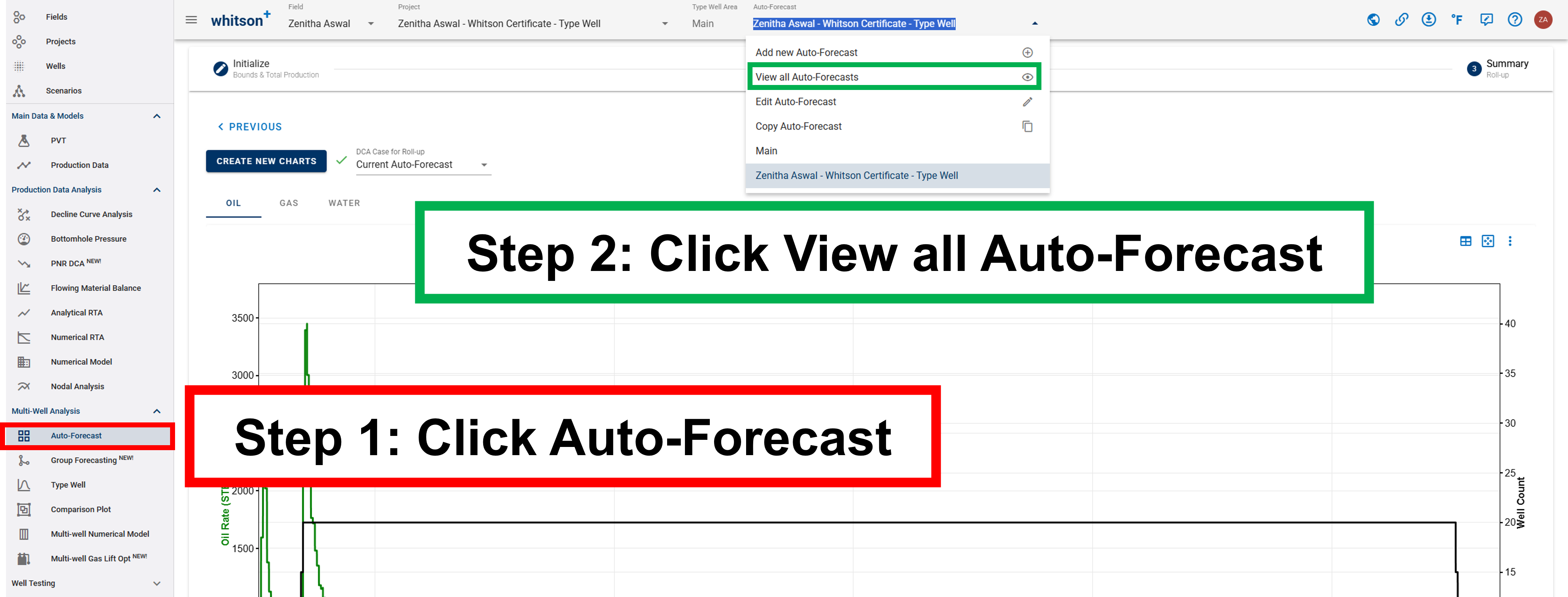
To return to the Auto-Forecast overview, either: 1. click the Auto-Forecast tab in the navigation panel. 2. or click the Auto-Forecast menu in the top bar.
4. Want to edit Auto-Forecast well selection?
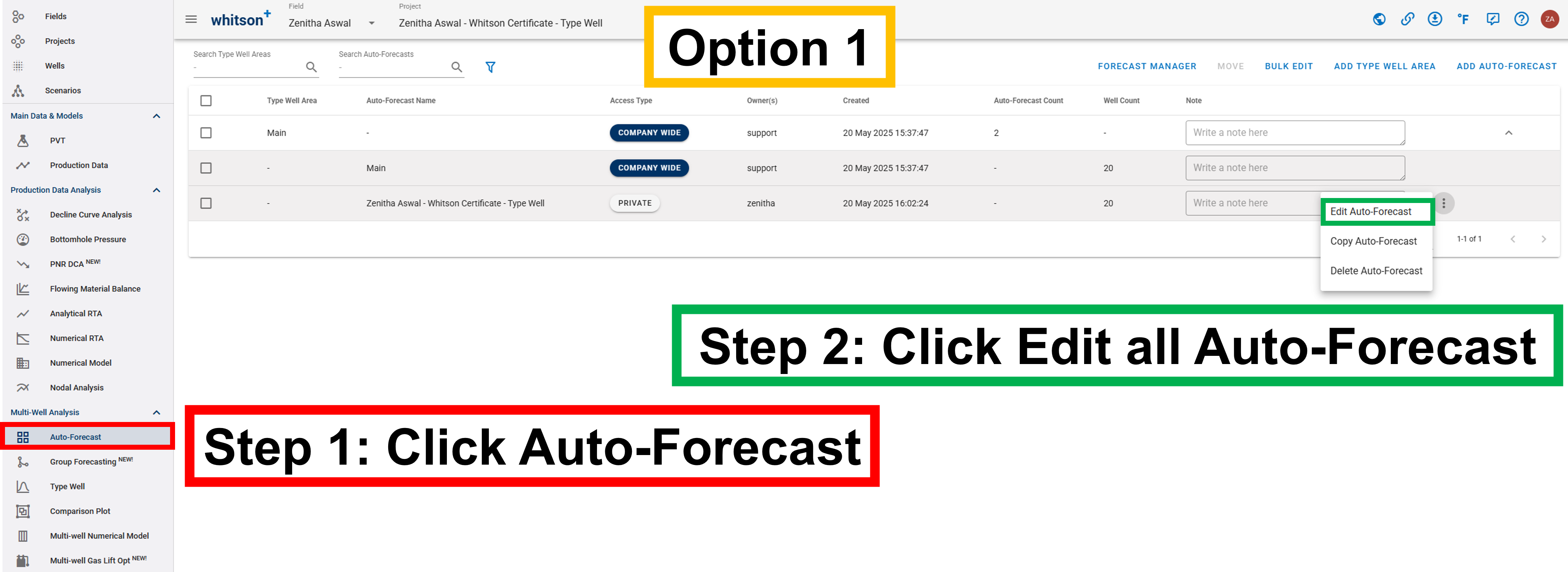
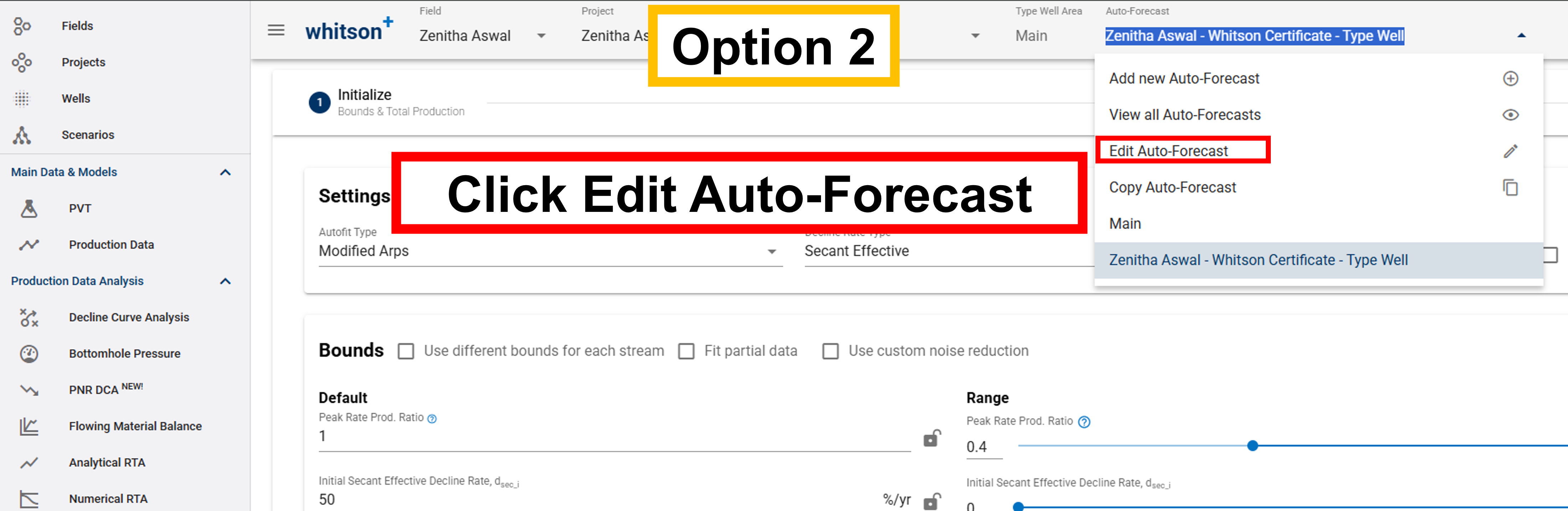
To edit the well selection, either:
- click the Edit Auto-Forecast tab in the Auto-Forecast Overview.
- or click the Edit Auto-Forecast menu in the top bar.
Decline Curve Analysis
Decline curve analysis (DCA) for all three flowing phases can be performed within whitson+, both automatically and manually. User-friendly drag-and-drop curve-fitting functionality is also available.
1. Input
The inputs for this analysis are:
- DCA parameters (\(b\), \(a_i\), \(q_i\))
- Start (day or month)
- Total production period (years)
- Limited Decline Rate (\(a_{lim}\) or \(d_{lim}\)). The user can decide whether to lock in the start day and the DCA parameters, or if these should change freely during the curve fitting.
2. Theory
2.1. Arps Fundamentals
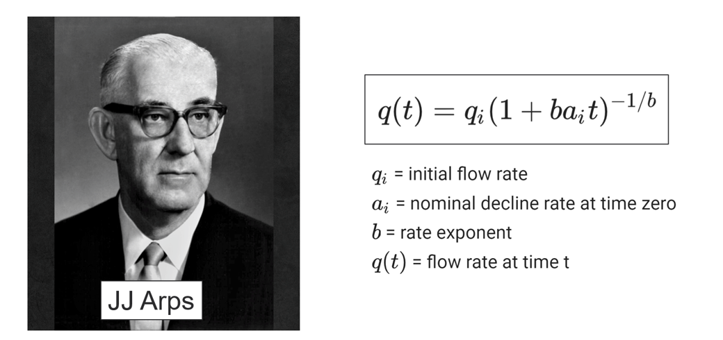
The classical equation that provides that basis for this module is
where
\(q_i\) = initial flow rate
\(a_i\) = nominal decline rate at time zero
\(b\) = rate exponent
\(q(t)\) = flow rate at time t
Equation 1 is a three-parameter performance-matching equation. When the \(b\) is equal to zero, the flow rate decline is exponential; when \(b\) is 1, the rate decline is called harmonic; and when b is between zero and one, the rate decline is hyperbolic.
2.1.1. Exponential Decline (b = 0)
where \(N(\infty)\) is the ultimate cumulative production.
2.1.2. Hyperbolic Decline (0 < b < 1)
2.1.3. Harmonic Decline (b = 1)
2.1.4. Beyond Hyperbolic (b > 1)
2.2. Other Segment Types
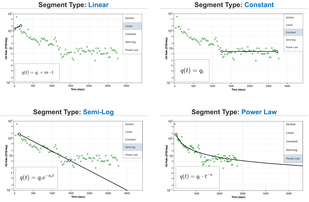
2.2.1. Linear
2.2.2. Constant
2.2.3. Semi-log
2.2.4. Power Law
2.3. DCA Summary
| Type | Decline Rate | Producing Rate, q | Elapsed Time, t | Cum. Production, \(Q_{t}\) |
|---|---|---|---|---|
| Exponential | \(a_t = ln(\frac{q_i}{q_t})/t\) | \(q_ie^{-a_it}\) | \(ln(\frac{q_i}{q_t})/a_i\) | \(\frac{q_i-q_t}{a_i}\) |
| Hyperbolic | \(\frac{a_i}{a_t} = (\frac{q_i}{q_t})^b\) | \(q_i(1+ba_it)^{-1/b}\) | \(\frac{(q_i/q_t)^b-1}{ba_i}\) | \(\frac{q_i}{a_i(1-b)}(1-\frac{q_t}{q_i}^{1-b})\) |
| Harmonic | \(\frac{a_i}{a_t} = \frac{q_i}{q_t}\) | \(q_i(1+a_it)^{-1}\) | \(\frac{(q_i-q_t)}{a_iq_t}\) | \(\frac{q_i}{a_i}ln(\frac{q_i}{q_t})\) |
| Linear | \(a_t = \frac{-m}{q_t}\) | \(q_i + m t\) | \(\frac{q_t - q_i}{m}\) | \(\frac{1}{m} \left[q_i(q_t - q_i) + \frac{(q_t - q_i)^2}{2}\right]\) |
| Constant | \(a_t = 0\) | \(q_i\) | \(t\) | \(q_i t\) |
| Semi-Log | \(a_t = ln(\frac{q_i}{q_t})/t\) | \(q_ie^{-a_it}\) | \(ln(\frac{q_i}{q_t})/a_i\) | \(\frac{q_i-q_t}{a_i}\) |
| Power-Law | \(a_t = n \left(\frac{q_t}{q_i}\right)\) | \(q_i \left(\frac{q_i}{q_t}\right)^n\) | \(t = \left(\frac{q_i}{q_t}\right)^{1/n}\) | \(\frac{q_i}{1-n} \left[\left(\frac{q_i}{q_t}\right)^{\frac{1-n}{n}} - t_0^{1-n}\right], \text{ if } n \neq 1\) or \(\frac{q_i}{n} \ln\left(\frac{q_i}{q_t}\right) - q_i \ln(t_0), n = 1\) |
| Type | Cumulative Production | Cumulative Production (with time substituted) |
|---|---|---|
| Exponential | ||
| Hyperbolic | ||
| Harmonic | ||
| Linear | ||
| Constant | ||
| Semi-Log | ||
| Power-Law | or | or |
Incline Auto Fit Type
The Incline segment in Auto Fit is based on the same Arps equations used for traditional decline curve analysis, i.e.: harmonic, hyperbolic, and exponential.
What distinguishes it is that it uses a negative nominal decline rate at time zero (aᵢ) and a negative rate exponent (b), allowing the model to capture inclining production rates.
2.4. Decline Rate Type
Mixed Effective Decline Rate
The Mixed Effective decline rate type is the default option in whitson+. It combines both secant and tangent effective decline definitions.
For this decline type:
- The initial effective decline rate is interpreted using the secant effective formulation (effective hyperbolic decline).
- The limiting effective decline rate is interpreted using the tangent effective formulation (effective exponential decline).
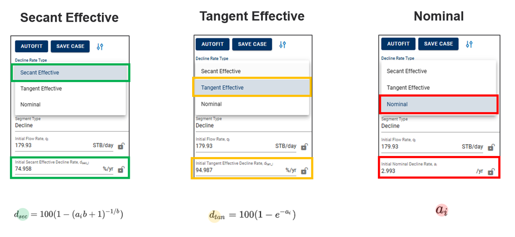
Nominal annual decline rate is denoted "a". The effective annual decline rate is denoted "d", with units %/yr. There are two common ways the industry converts annual decline into effective decline,
"Secant Effective" aka "Effective Hyperbolic Decline"
"Tangent Effective" aka "Effective Exponential Decline"
Both of these properties can be converted back by the following equations
Note
These numbers are mere conversions to and from \(a_{i}\) and should yield identical results irrespective of what is chosen. For most folks, it's mainly the matter of preference when it comes to what is communicated in terms of the final results.
The symbols for the different terms can vary somewhat from software to software, so here is a little overview for some handpicked softwares.
| Name | whitson+ | ARIES | Harmony | PHDWin / MOSAIC / SPEE | Val Nav |
|---|---|---|---|---|---|
| Initial nominal annual decline rate | \(D_{i}\) | \(A_{i}\) | \(a_{i}\) | \(D_{i}\) | Di (nom) |
| Secant effective annual decline rate | \(D_{esi}\) | \(D_{b}\) | \(d_{i,sec}\) or \(d_{lim,hyp}\) | \(D_{esi}\) | Di (eff. sec) |
| Tangent effective annual decline rate | \(D_{ei}\) | \(D_{h}\) | \(d_{i,tan}\) or \(d_{lim,exp}\) | \(D_{ei}\) | Di (eff. tan) |
| Rate exponent | b | n | b | b | Ni |
2.5. Effective Decline: Secant vs Tangent
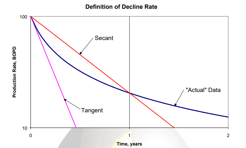
The decline rate is not constant but changes with time because the data are plotted as a curve on semi-log paper.
The hyperbolic decline rate is the rate of change of the decline rate with respect to time, or the second derivative of the production rate with respect to time.
There are three ways to define the initial decline rate for hyperbolic decline: nominal, tangent effective, and secant effective.
The figure above illustrates the difference between the tangent effective and secant effective definitions of the initial decline rate.
More information about this is provided by SPEE.
2.6. Limited / Modified Decline
The limited decline rate begins when the hyperbolic decline curve transitions into an exponential decline curve at a specified limiting effective decline rate (\(d_{lim}\)). The limiting effective decline rate is converted to a limiting nominal decline rate (\(a_{lim}\)), and the following equations are applied:
When \(d_{tan}\) > \(d_{lim}\):
when \(d_{tan}\) <= \(d_{lim}\):
where
which, also can be simplified into:
2.7. Plot Settings and Straight Lines
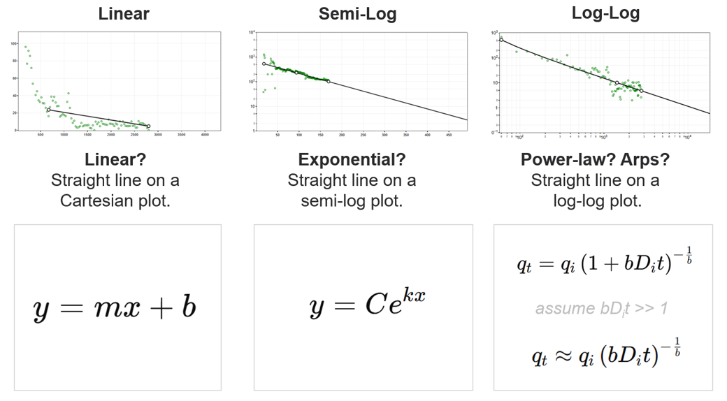
Linear, Semi-Log, and Log-Log plots provide distinct visualizations for identifying decline behavior and interpreting reservoir characteristics. Each plot highlights specific relationships between production rate and time or cumulative production.
-
Linear: A straight line on a Cartesian plot. Useful for identifying constant-rate declines or linear trends.
-
Semi-Log: A straight line on a semi-log plot. Exponential declines, which are often typical of fluid-flow-dominated regimes, become linear in this format.
-
Log-Log: A straight line on a log-log plot. Power-law declines, such as those observed in fractured reservoirs, are best visualized using this plot.
2.7.1. Why Do Linear Segments Look Curved in Rate-Cumulative Space?
A linear segment defined in rate-time space, such as , appears curved in rate-cumulative space because cumulative production is calculated by integrating the production rate over time.
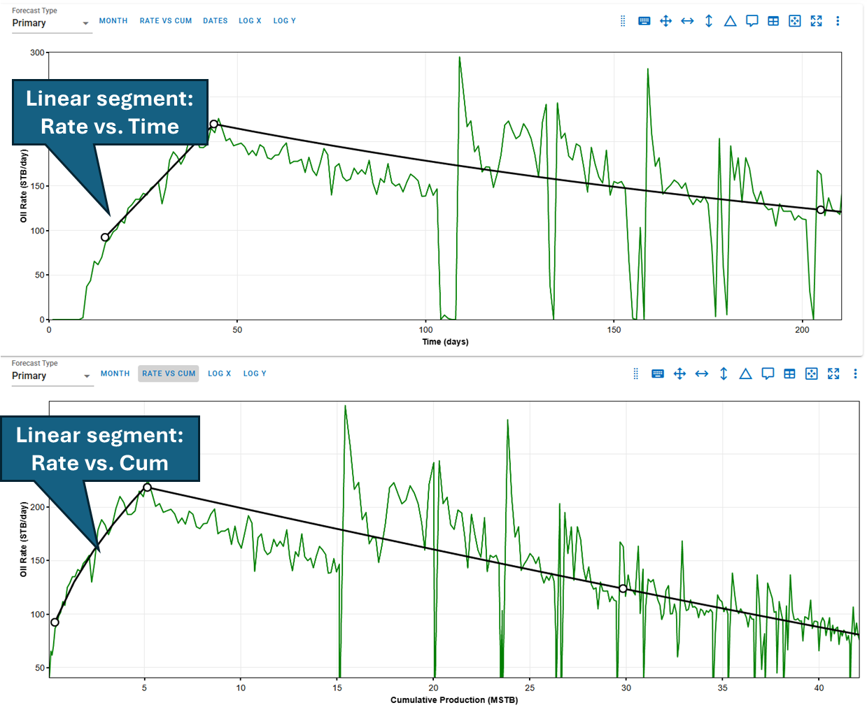
Cumulative is given by:
To convert to rate-cumulative space (i.e.,), you must solve this nonlinear equation for and substitute back into , resulting in:
Because involves a square root, the final expression for is curved — even though is a straight line. This applies both for declining and increasing (buildup) segments.
2.8. Fetkovich
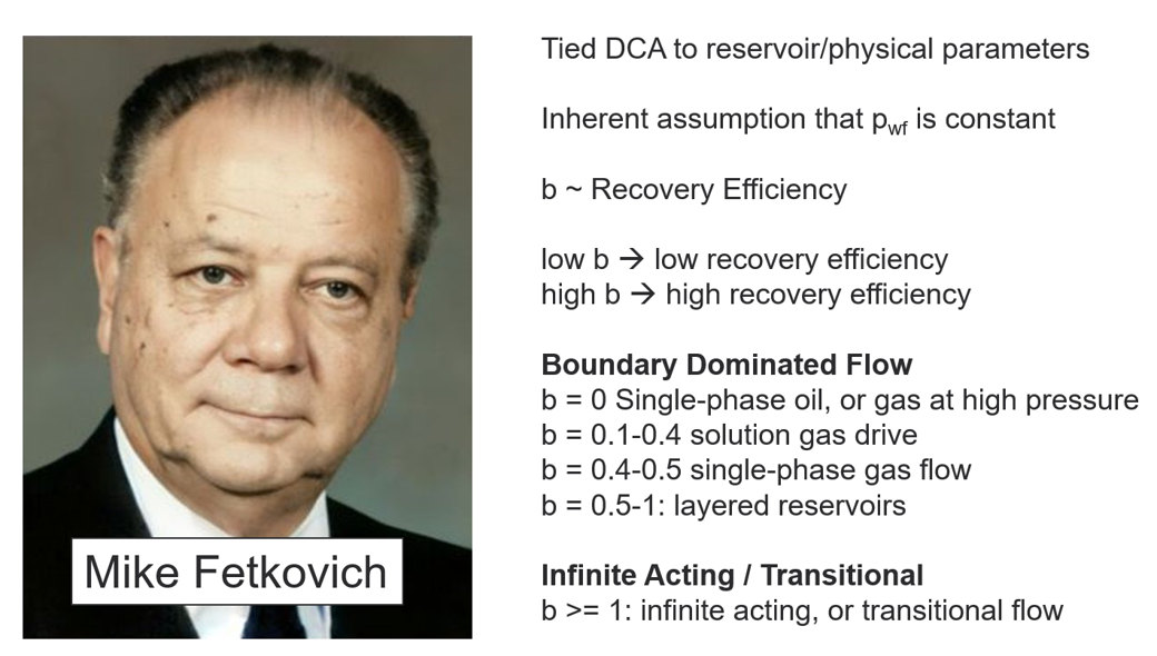
Mike Fetkovich advanced Decline Curve Analysis (DCA) by linking it directly to reservoir and physical parameters, with the b-factor playing a central role in this approach. For the b-factor to have physical significance, it must be derived while the well is producing under near-constant bottomhole pressure. The b-factor serves as an indicator of recovery efficiency, or reservoir "energy." A low b-factor signifies a low-energy system with lower recovery efficiency, while a high b-factor represents a high-energy system with greater recovery potential. The table below provides general guidelines for interpreting the b-factor and its relationship to reservoir characteristics.
| \(b\) value | Context |
|---|---|
| 0 | Single-phase oil, or single-phase gas at high pressure |
| 0.1 - 0.4 | Solution gas drive |
| 0.4 - 0.5 | Single-phase gas flow |
| 0.5 - 1 | Layered reservoirs |
| > 1 | Infinite acting flow |
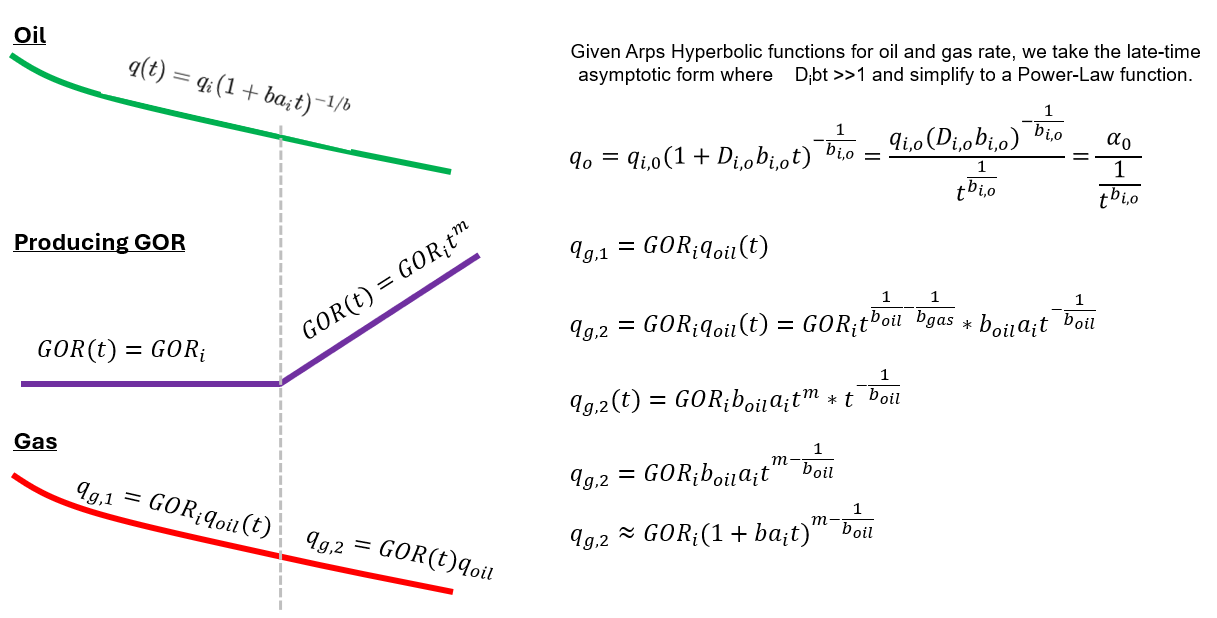
2.9. Ratio Forecasting
2.9.1. Changing Forecast Type
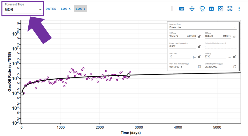
You can switch from considering the primary phase (oil, gas, or water) to using a ratio forecast type. For example, if you perform segment fitting using GOR for oil, the forecast will use the resulting GOR profile and multiply it by the gas profile to obtain the forecasted oil rate profile.
2.9.2. Derivation: Why should Ratios be Power-Law?
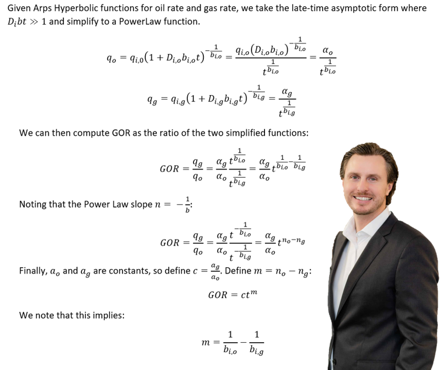
2.9.3. How to convert Power-Law to Arps?
For further information, please refer to [1].
2.10 Arps and Derivatives
Arps decline parameters can be expressed directly in terms of derivatives of production rate. The instantaneous decline parameter \(D\) is also called the loss-ratio, and \(b\) is the derivative of the loss-ratio \(1/D\).
The rate-time definitions are:
Alternatively, the same parameters can be derived in rate-cumulative space:
where \(q\) is production rate, \(t\) is time, and \(Q\) is cumulative production. For a declining well, \(dq/dt < 0\), so \(D > 0\).
This concept in practice
The derivative-based definitions of \(D\) and \(b\) are a convenient way to compute decline behavior directly from production data without assuming a specific decline curve form upfront. Reese et al. (SPE-171568-MS) use these relationships to track how \(b\) can evolve through time in MFHW shale wells (e.g., during and after linear flow), and they demonstrate how multi-segment Arps forecasts can better represent those flow-regime transitions than a single fixed \(b\) value.
3. Decline Curve Analysis in whitson+
3.1. Autofit
The autofit algorithm finds the last segment of the data that is continuously non-zero and fits the DCA parameters to only that portion of the data. A single zero rate or a series of consecutive zero rates in the data is typically associated with a shut-in, after which the DCA fit should be reinitialized.
3.1.1. Residual Function
The fitting routine uses the following residual function in the least square routine.
where \(r_i\) is the residual at time \(i\), \(w_i\) is the weight factor of time \(i\), \(t_0\) is the time index and q is the actual rate.
3.1.2. Default Bounds
| Parameter | Lower Bound | Higher Bound | Unit |
|---|---|---|---|
| \(q_i\) | 40% of max observed q | 20% higher than max observed q | volume unit / time |
| \(a_i\) | 0 | 10 | /yr |
| \(b\) | 0 | 2 | - |
3.1.3. Adjusting default autofit bounds on DCA parameters
Settings Adjustment
You can also adjust the settings for autofitting decline to your data by adjusting the decline parameter ranges and specifying the autofit type as the default modified Arps decline.
The Autofit function will automatically switch to exponential decline when it reaches the limiting decline rate. If the Autofit type is set to Modified Arps, it will fit two segments to the data by default. You can choose to autofit some or all segments at once, and control autofitting for each segment individually using the locks on the decline parameters.
3.1.4. Weighting factors
By default, all days have a weighting factor of 1, except from the days when q = 0, in which the weighting factor is 0.
3.2. DCA on physics-based forecasts
If a physics based forecast has been established for this well via the numerical model, an option to include this data will appear as a toggle, shown below.
You can build a physics-based forecast using the Numerical Model feature, where the reservoir simulation history matches the well and generates a forecast based on your model setup.
Once the model is simulated with a forecast included, you can import the history match into the DCA feature. This allows you to build decline curves for the simulated data—including the forecast—enabling physics-based DCA forecasting.
3.3. General tips
3.3.1. Manually adjusting DCA parameter graphically
In whitson+, users can manually adjust specific points on the DCA plot, each influencing different parameters that define the production decline trend.
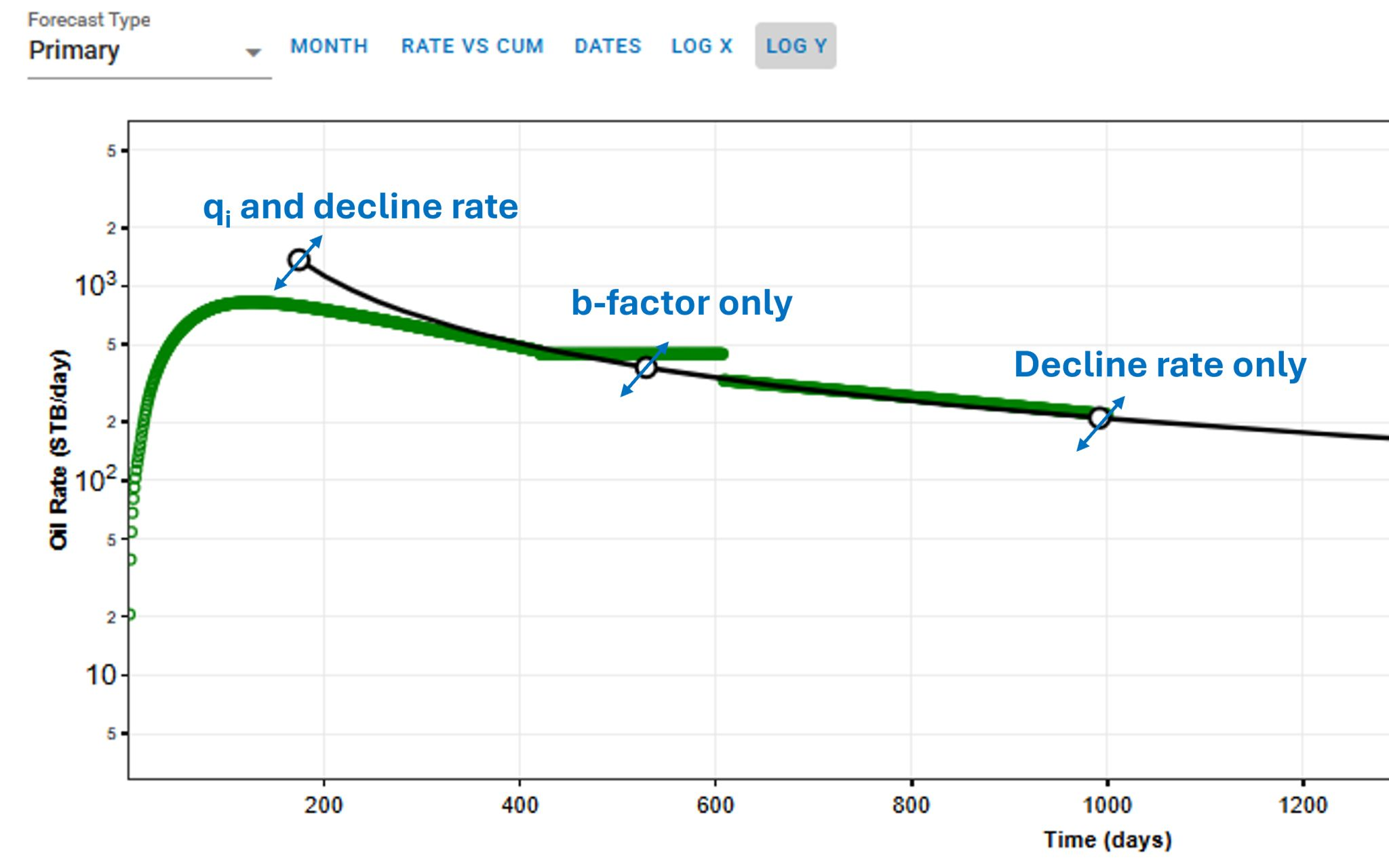
Adjustment points:
- First point: modifies both the qi and decline rate. This adjustment impacts the early production and the overall scale of the decline curve.
- Second point: adjusts the b-factor only, which controls the curvature of the decline trend. A higher b-factor leads to a slower decline in production, while a lower b-factor results in a steeper drop.
- Third point: alters only the decline rate, influencing the rate at which production decreases over time.
Why manual adjustments matter?
Manually refining these parameters allows users to create more accurate production forecasts, particularly in unconventional reservoirs where decline trends may not fit standard analytical models perfectly. This flexibility helps in optimizing well performance analysis and forecasting long-term production more effectively.
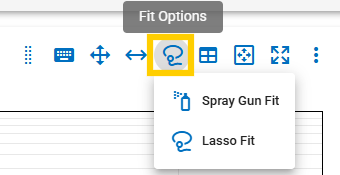
3.3.2. Fit forecasting data points
When utilizing the Lasso or Spray Fit tools to perform DCA forecasting, a subset of the available data points is selected based on the user-defined lasso or spray selection area.
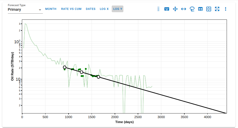
After the selection and fit are performed:
- The selected data points are visually differentiated by being displayed in a distinct color on the plot.
- The non-selected data points remain in the background, ensuring clear visual distinction between included and excluded data.
This visual feedback allows users to:
- Quickly review which data points were used for the forecast generation.
- Validate the forecast by checking if the selected data appropriately represents the well's production history or expected future trend.
- Identify and exclude anomalies or non-representative periods, such as operational changes, shut-ins, or erratic production behavior, by adjusting the selection.
3.3.3. Adding multiple decline segments
You can add multiple Arps decline segments to the data, as proposed by the Modified Arps decline method (2 segments). Each of these segments can be linear incline, constant or the Arps decline type segments - controlled individually by directly entering the inputs, or adjusting the curve on the plot itself to auto-compute the decline parameters for each of them.
Note
Adding multiple segments may be useful to model particular flow regimes, constant rate well control or refrac analysis.
3.3.4. Where does the DCA forecast append to historical data?
The end date of the forecast on the DCA plot dictates where the forecast is appended to historical data.
The forecast is appended at the earlier of:
-
the last producing day in the well’s history, or
-
the end date of the last forecast segment.
The EUR is calculated based on this setup:
-
If the forecast end date is beyond the last producing day, the entire production history is included, followed by the forecast, to compute the EUR.
-
If the forecast end date is before the last producing day, the forecast is appended from that date onward, and any actual production data after this date is ignored in the EUR calculation.
EUR shown in the top-left box should be exactly equal to the EUR (black line) plotted on the cumulative plot (bottom) at the end of the total production period.
3.3.5. Historical Cummulative Production in DCA
The cumulative production values—Np (oil), Gp (gas), and Wp (water)—are calculated from the first day of recorded production up to the start of the forecast period. These values represent historical (actual) cumulative production for each phase.
There are two possible scenarios depending on the segment-fit end date:
-
Segment-fit end date is before the last historical production date
In this case, the historical cumulative (Np, Gp, Wp) is calculated only up to the segment-fit end date, as the forecast begins before the end of available production data.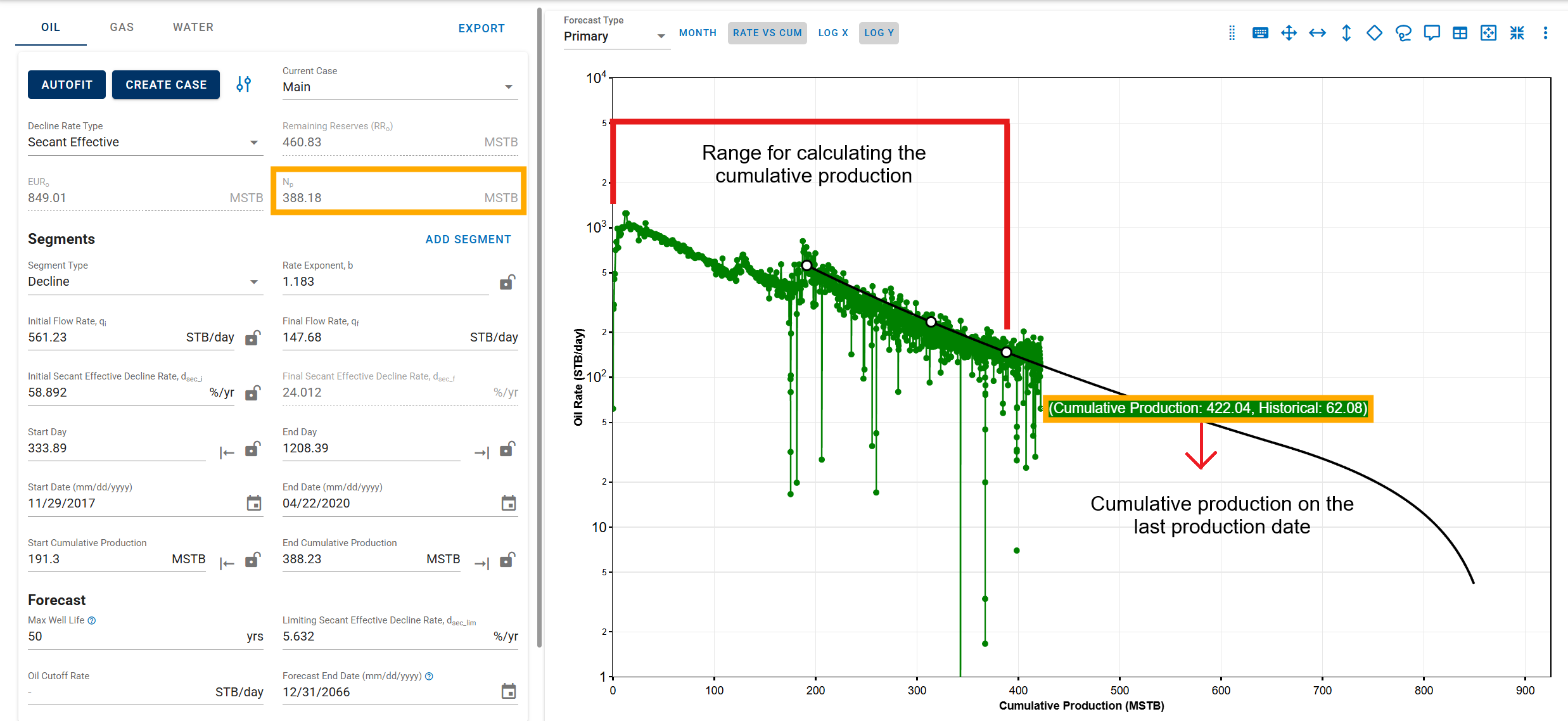
-
Segment-fit end date is after the last historical production date
Here, the historical cumulative values include all available production data up to the last recorded date, and the forecast begins from that point forward.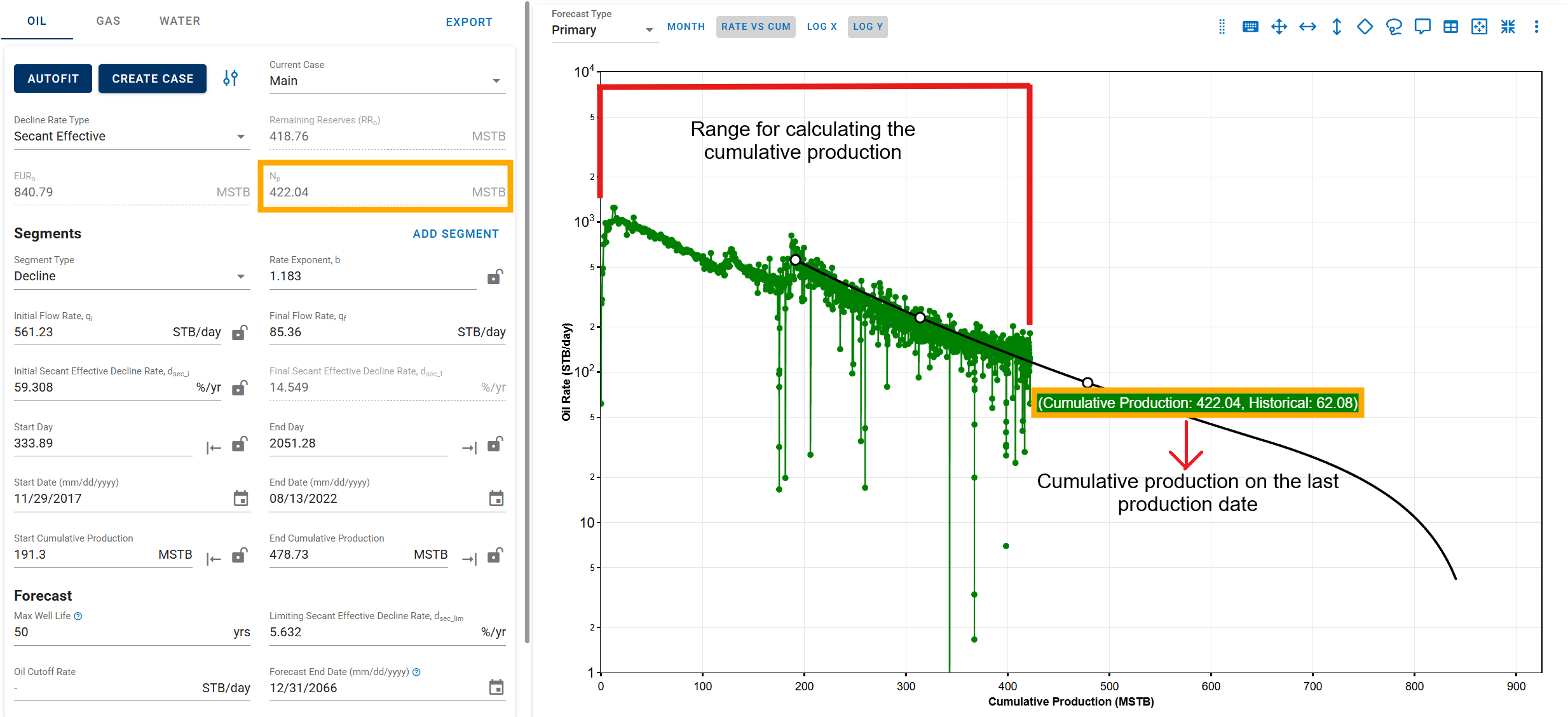
3.3.6. Rate-time decline vs Rate-cum decline
You can observe the decline fit in rate vs time space or rate vs cumulative space on the same plot (top).
3.3.7. Converting from Rate-Cum to Rate-Time
When transitioning betweem rate-cum and rate-time domains in DCA, it is essential to perserve consistency, particulartly with Estimated Ultimate Recovery (EUR). However, the relationship between rate, time, and cumulative production are nonlinear and sensitive to segment definition.
To maintain the same EUR in both spaces, whitson+ performs a back calculation of the initial segment parameters when switching between domains.
Rate-Cum:
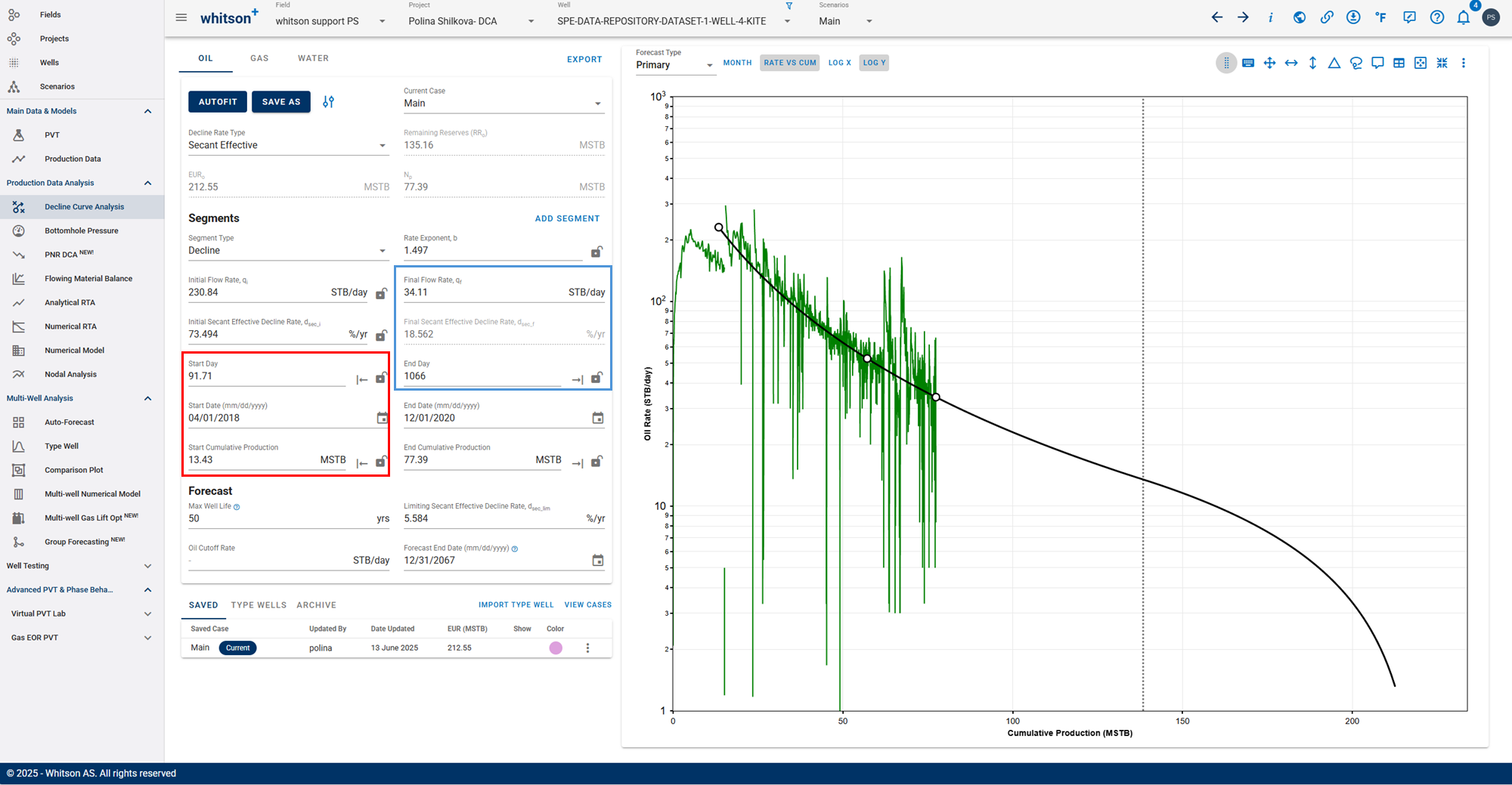
Rate-Time:
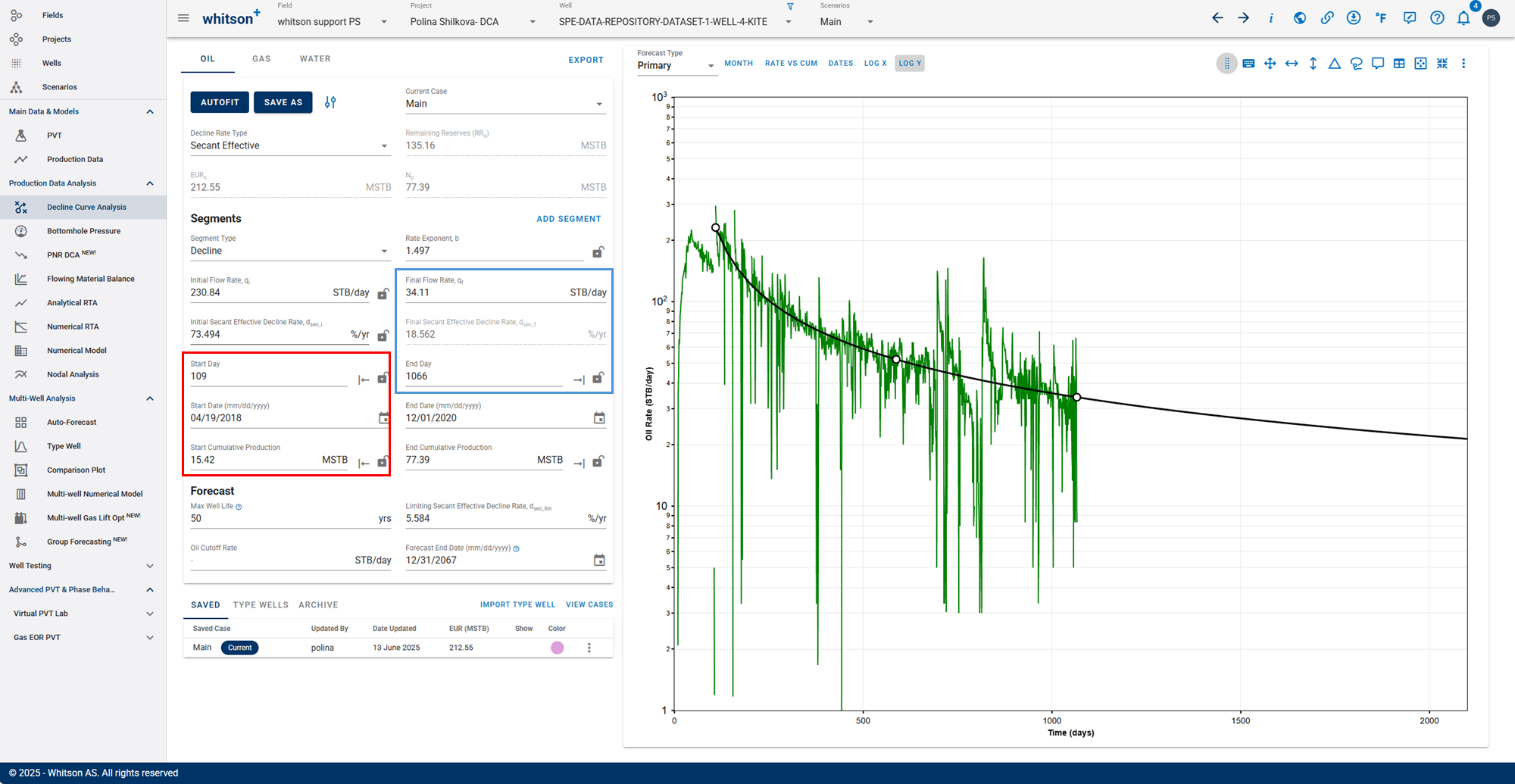
- The forecast end parameters (marked in blue) remain fixed.
- The segment start parameters (marked in red) are recalculated when switching between domains to ensure that cumulative production and EUR remain consistent.
This approach ensures that the cumulative production curve integrates correctly over time, regardless of whether the input is in rate-time or rate-cum space.
Practical Implication
Switching between rate-time and rate-cum in the DCA module automatically recalculates the segment start or end parameters depending on which domain is active, while holding EUR constant.
This ensures:
1. EUR stability between views
2. Accurate forecast matching
3. Avoidance of manual tuning when switching domains
3.3.8. Linking decline segments
You can use the 'Link to Previous Segment' checkbox for each segment to link the previous segment to this one in time for continuity.
The 'Link Decline Rates' function ensures continuity in both production rates and decline behavior between two consecutive decline segments in a segmented DCA (Decline Curve Analysis) model.
When the Link to Previous Segment checkbox is selected:
-
The start rates of the current segment (e.g., oil, gas, water) are automatically set to match the end rates of the previous segment.
-
The initial decline parameters of the current segment are computed to ensure a smooth transition from the previous segment.
-
This removes discontinuities and manual adjustments, resulting in a more realistic and physically consistent forecast.
3.3.9. Saving the DCA fit
You can save your current DCA fit as a Saved Case using the Save Case button. This allows you to create a checkpoint of your current fit before making further adjustments.
Key Features:
-
Use the Save Case button to store the current set of DCA parameters.
-
Saved cases can be visualized on the DCA plot by checking the box under the "Show" column next to each saved case.
-
To restore a previously saved DCA fit, click the three vertical dots next to the case and select Load Case.
-
If you try to save a case using a name that already exists, the system will prompt you to confirm whether you want to overwrite the existing case.
Importing saved Type well DCA case to DCA and saved cases from DCA into Type well
If you fit DCA to the type well, made from a set of wells in the Type Well feature (DCA tab), and save that, you can import this saved DCA fit for the type well into list of saved cases in this feature. This lets you plot your type well decline over the actual well decline to compare.
Alternatively, if you saved the DCA fits for all the wells with the same name, you can import this into the Type well feature such that each of the individual well declines set up with that name is appended to the respective wells and the Type well is built for historical data + individual well declines. This removes the need for forecasting the constructed type well with DCA.
3.3.10. Assigning multiple type wells
In whitson+, there is no restriction on the number of type wells that can be imported and stored within a project. This flexibility enables users to conduct more robust benchmarking and performance evaluation of individual well forecasts against various type well scenarios.
For any single well with a forecast, users can:
- Import multiple type wells to the module.
- Assign and compare these type wells to the well's DCA forecast.
- Visually overlay the DCA forecast and type wells on the same plot.
This feature is particularly useful when:
- Evaluating well performance against AFE (Authorization for Expenditure) or pre-drill expectations.
- Comparing with prior forecasts or updated type wells to track performance over time.
Each well is associated with one "main" type well, which serves as the default, however:
- Multiple type wells can be loaded concurrently for side-by-side comparisons.
- All associated type wells remain stored and accessible for future evaluations.
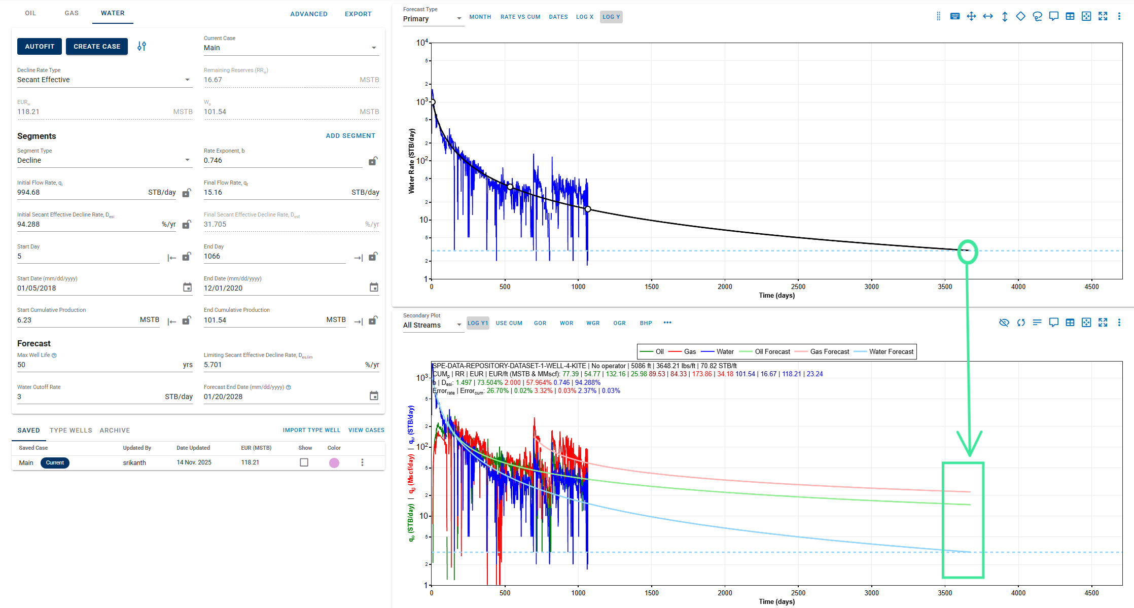
3.3.11. Linked Forecast End Dates Across Phases
The forecast end date for any of the oil, gas or water phase DCA will occur based on the limitation reached for that phase, that is informed by the provided “Max Well Life” or “Cutoff Rate” (whichever comes first). However, the forecast end date is independent of the other phases or in other words, is not linked to the other phases, only when the case name across the phases is different.
When the case names are the same across the phases, their forecast end dates get linked. Whichever phase reaches its forecast limit first in time, the DCA for the other phases also terminate at the same time limit.
In the case shown below, the end date for the water forecast in the “Main” case reaches first, thus limiting the “Main” case forecasts for Oil and Gas to the same time limit.
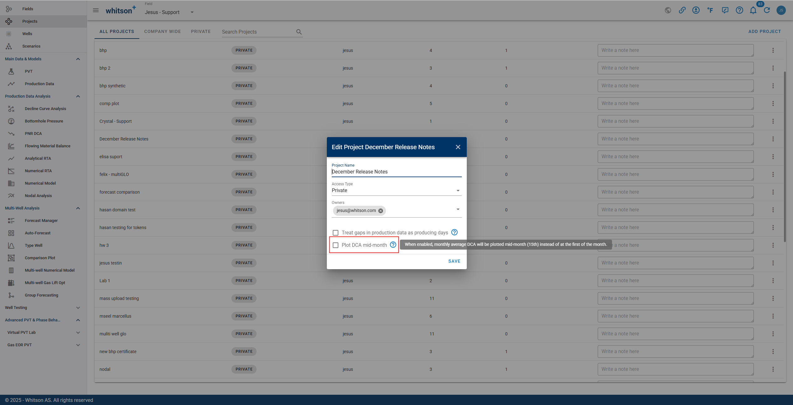
3.3.12. Plot DCA mid-month
For wells with monthly production data, whitson+ can plot DCA rates on the mid-month date (15th) instead of the uploaded first or end-of-month date. This is controlled by a project-level setting and helps make monthly points align more intuitively on time-series plots.
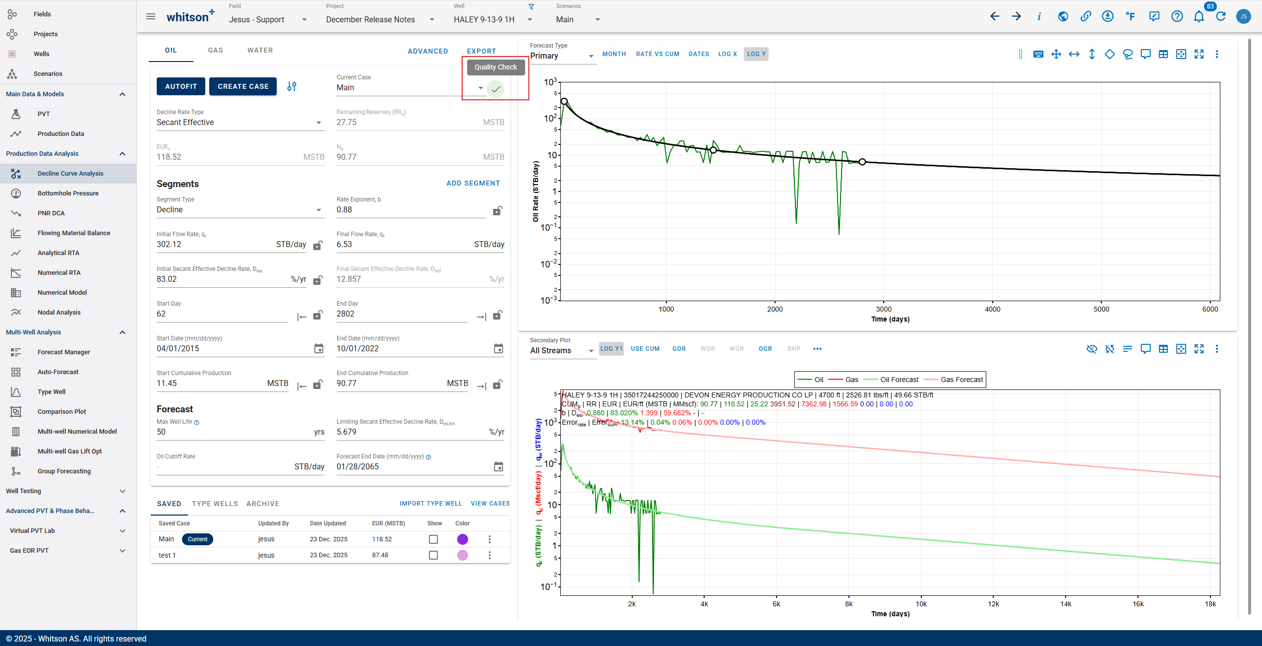
3.3.13. DCA quality checks
Forecasts can now be marked with a quality check status:
- undone
- bad
- moderate
- good
This status is available across Auto-Forecast, Bulk View, and single-well DCA, and it can also be used as a sortable field in Forecast Manager to help QC and prioritize wells.
3.4. Hotkeys
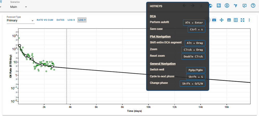
The following hotkeys are available to streamline your workflow and enhance navigation within the software:
3.4.1. Decline Curve Analysis (DCA)
- Perform Autofit: Press
Alt + Enterto automatically fit the decline curve to the available data. - Save Case: Use
Ctrl + Sto save the current case, ensuring no changes are lost.
3.4.2. Plot Navigation
- Shift Entire DCA Segment: Hold
Altand drag the mouse to shift the entire decline curve analysis segment on the graph. - Zoom: Click and drag the mouse over a region to zoom into specific areas of the plot for detailed analysis.
- Reset Zoom: Double-click anywhere on the plot to reset the zoom level to the default view.
3.4.3. General Navigation
- Switch Well: Use
PgUp/PgDnto move between wells in the dataset. - Cycle to Next Phase: Press
Shift + Sto cycle between different production phases. - Change Phase: Use
Shift + O/G/Wto switch between oil, gas, and water phases.
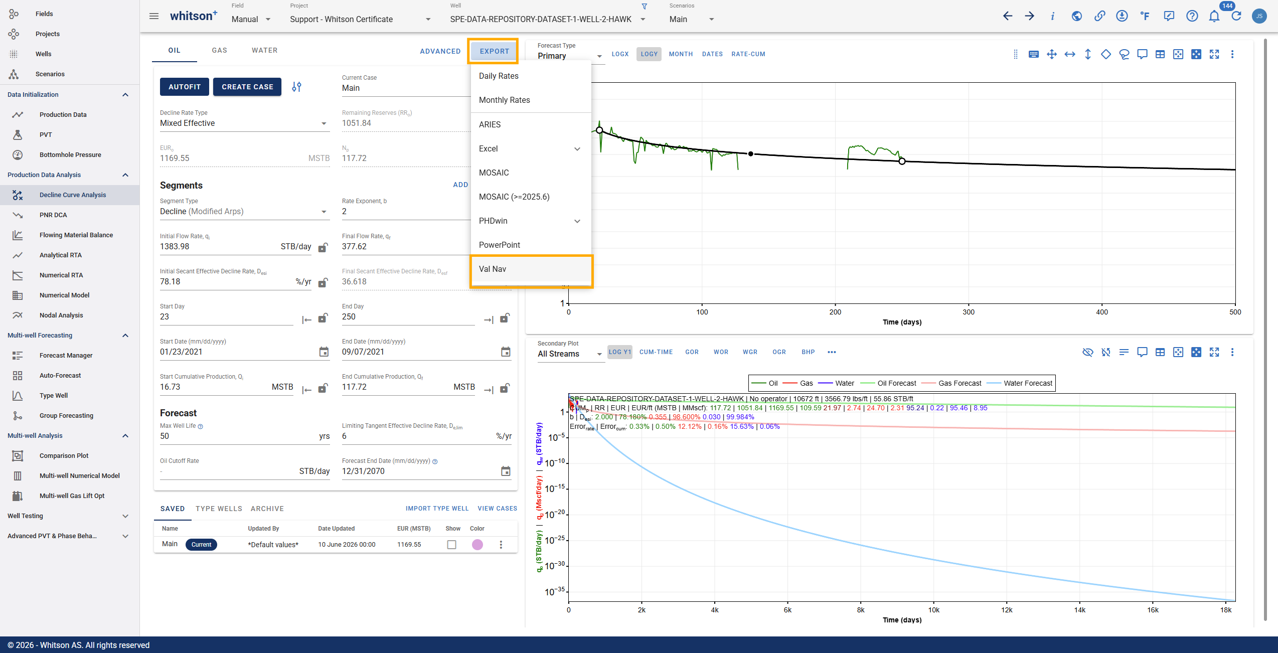
4. Export
The results from the DCA feature can to be exported to:
- Aries
- ComboCurve
- Excel
- PHDWin
- Mosaic
- Val Nav
Note that the forecast in the export starts from the end of the uploaded historical data. Hence the best fit qi and decline parameters has to be recalculated for the end of history (as they change with time), as outlined here.
PHDWin: Uses Secant Effective or Tangent Effective Decline?
PHDWin uses Initial Tangent Effective Decline Rate.
4.1. ARIES
4.1.1. Aries Examples
The following outlines how the ARIES export works with a specific example.
For an example well with these parameters.
- qi = 51.7334 STB/d
- d_lim = 5.0000 %/yr
- b = 1.2
- d_sec = 43.7863 %/yr
- Cutoff rate = 3.0 STB/d
- forecast_time = 582.3934 months
There will be 4 cases, these are all shown assuming the parameters are for the oil phase, but the logic is equally applicable for gas and water.
Case 1 - well reaches cutoff rate before d_lim, the ARIES export would look like this:
We have a single line which shows qi, cutoff rate, b and d
DEMOWELL
PRODUCTION
CUMS 80.1645 0.4055 780.3532
START 03/2022
OIL 51.7334 3.0 B/D X MOS B/1.2 43.7863
Case 2 - well reaches cutoff rate after d_lim but before end of forecast period, the ARIES export would look like this:
We have two lines as before, only difference being that instead of putting the period of 582 months (or any number for the case), we put X
DEMOWELL
PRODUCTION
CUMS 80.1645 0.4055 780.3532
START 03/2022
OIL 51.7334 X B/D 5.0000 EXP B/1.2 43.7863
" X 3.0 B/D X MOS EXP 5.0000
Case 3 - well reaches d_lim and does not reach cut off rate until the end of the forecast period, the ARIES export would look like this:
DEMOWELL
PRODUCTION
CUMS 80.1645 0.4055 780.3532
START 03/2022
OIL 51.7334 X B/D 5.0000 EXP B/1.2 43.7863
" X X B/D 582.3934 MOS EXP 5.0000
Case 4 - d_sec is lower than d_lim:
In addition to these 3 main cases, there is an exceptional case in which d_sec < d_lim, for example if in the case presented above d_sec was 3.2561 %/yr instead 43.7863 %/yr. The export to Aries would look as follows.
Case 4a - If cutoff rate is not reached before end of forecast period:
DEMOWELL
PRODUCTION
CUMS 80.1645 0.4055 780.3532
START 03/2022
OIL 51.7334 X B/D 582.3934 MOS EXP 3.2561
Case 4b - If cutoff rate is reached before end of forecast period:
DEMOWELL
PRODUCTION
CUMS 80.1645 0.4055 780.3532
START 03/2022
OIL 51.7334 3.0 B/D X MOS EXP 3.2561
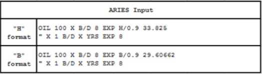
4.1.2. Aries: Secant Effective or Tangent Effective Decline?
In ARIES, the most commonly used format is 'secant effective,' also known as the 'B format.' This is what whitson+ will export to ARIES by default. However, there is also an option to use 'tangent effective,' referred to as the 'H format' in ARIES. Refer to the picture below to see the difference between these formats in ARIES.
4.2. PHDwin
Latest feature enables exporting DCA forecasts to PHDwin v3 format files, in addition to the previously supported PHDwin v2 format.
4.3. Val Nav
Option to export DCA results excel sheet in Val Nav import format for the selected saved case.
Here's some examples of what the export file from whitson+ would look like:
-
Val Nav Decline Import Template.xlsx
Import Notes Regarding Decline Template:
- Only the columns highlighted in green are required for every record.
- Header names must match the expected field names exactly.
- In each header cell, note the expected units of that field.
- Every product decline segment must include a start date, Qi, and three Arps parameters to be considered valid.
- For the first segment, both start date and Qi are required.
- For the second and later segments, if start date and Qi are left blank, they will automatically link to the previous segment’s end date and Qf.
- For the second and later segments, you can set Di Linked = True to link Di to the Df of the previous segment.
- All segments within the same product decline must be grouped together and sorted in ascending order by segment index (earliest segment first).
- All product declines within the same entity must also be grouped together, though the order of those grouped declines does not matter.
- Decline types for Di and Df (
nominal,effective tangent, oreffective secant) are interpreted according to the user’s active decline-type setting in their user options. - Slope type can be left blank if ratio declines are not being imported.
-
Val Nav Forecast Constants Import Template.xlsx
Import Notes Regarding Forecast Constants Template:
- Only the columns highlighted in green are required for every record.
- Column headers must be matched exactly as written.
- The Second row defines the unit system and available options, so it must also be matched exactly.
4.3.1. Importing into Val nav
Use Spreadsheet Import in Val nav to load decline or forecast-constant data from the whitson+ export template.
- Go to File > Import > Spreadsheet Import.
- Select the spreadsheet you want to import.
- In the import dialog, set Mapping to either Declines or Forecast Constants, depending on what you are importing.
- Choose the correct forecast destination, such as the appropriate Plan and Reserves Category.
- Set Header rows to 2.
- If the spreadsheet header names match the expected field names exactly, the remaining fields should auto-map automatically.
4.4. Benchmarking DCA in whitson+
Several benchmark decline curve analysis cases have been recreated in whitson+ based on a public GitHub repository. These benchmark cases are being evaluated across multiple DCA platforms, and whitson+ consistently delivers some of the most accurate estimates of expected recovery volumes.
You can explore these cases by visiting: whitson+ Forecast Comparison
5. DCA Error Calculations
In whitson+, error calculations for rate and cumulative production during Decline Curve Analysis (DCA) follow the standard Root Mean Square (RMS) error formulation as described here.
This section outlines how RMS is applied specifically in DCA, with emphasis on how rate and cumulative errors are computed.
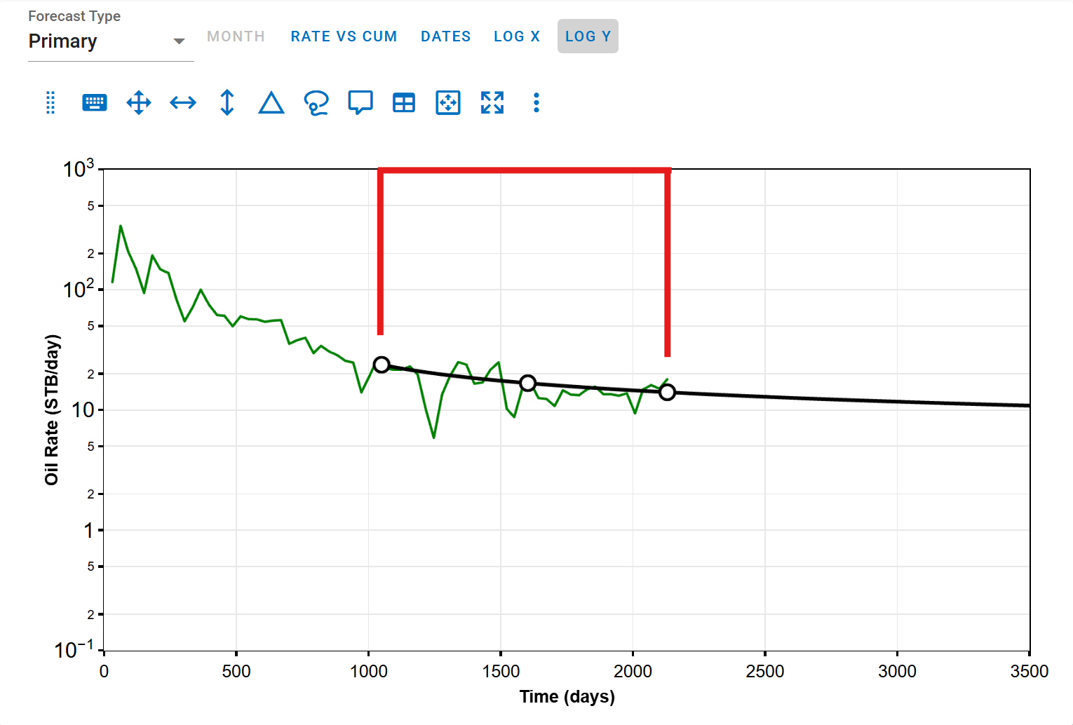
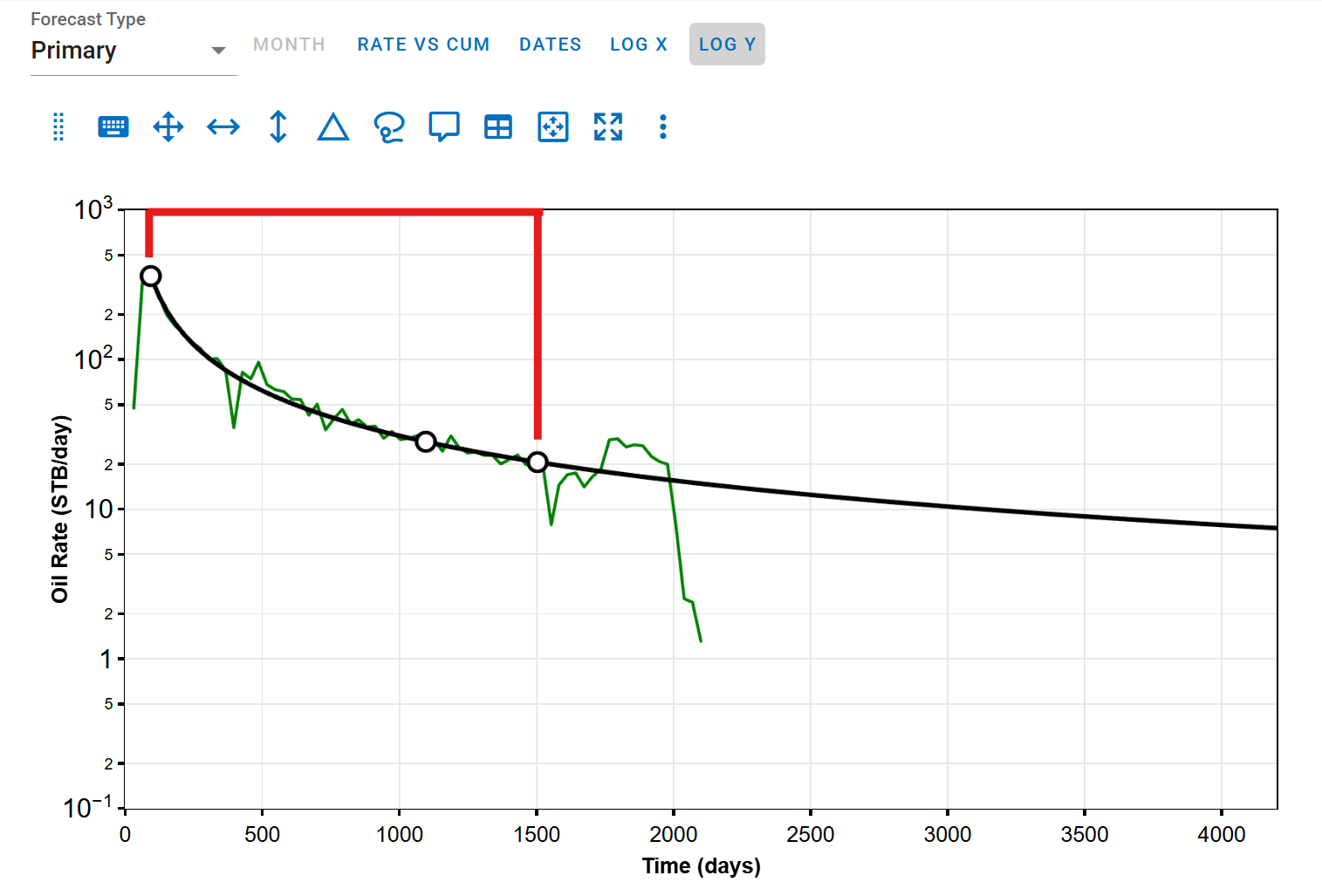
5.1. Rate Error
The rate RMS error is calculated using the difference between the historical rate data, and the forecasted rate from the DCA
By default, historical data points with zero rate are given a weight of 0 and are excluded from the error calculation.
Equation:
Where:
\(y_{i,\text{hist}} = \text{historical production value for observation} \text{ } 'i'\)
\(y_{i,\text{DCA}} = \text{forecasted DCA production value for observation} \text{ } 'i' \)
Examples:
The red-highlighted area indicates the range over which the RMS calculation is performed.
-
Forecast begins after history ends:
-
Forecast starts before history ends:
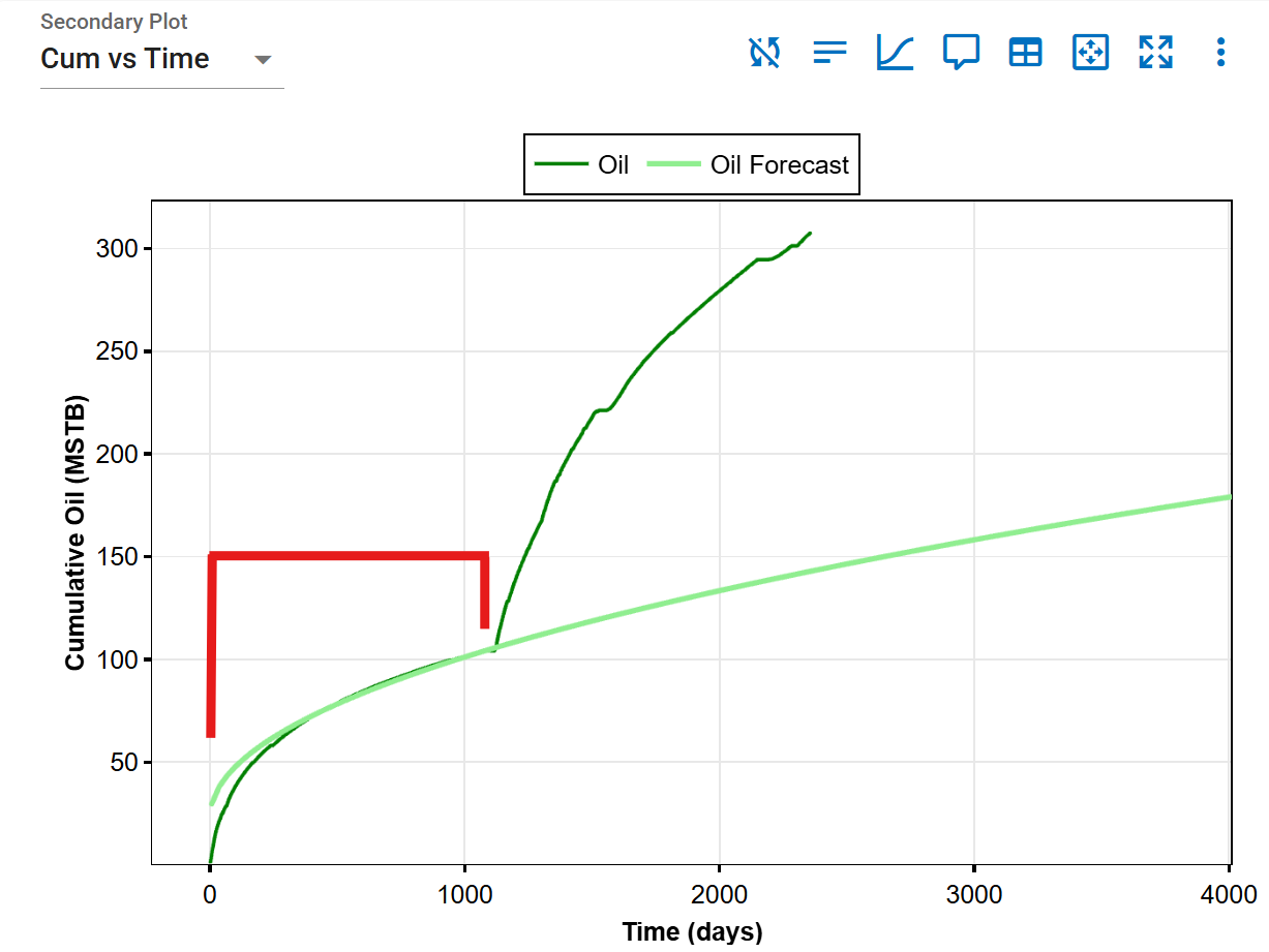
5.2. Cumulative Error
The cumulative error is calculated using the difference between the backcalculated forecast cumulative, and the historical cumulative data.
Equation:
Where:
\(y_{i,\text{hist}} = \text{historical cummulative data for observation} \text{ } 'i'\)
\(y_{i,\text{DCA}} = \text{forecasted DCA cummulative data for observation} \text{ } 'i' \)
Examples:
The red-highlighted area indicates the range over which the RMS calculation is performed.
-
Forecast starts at end of history:
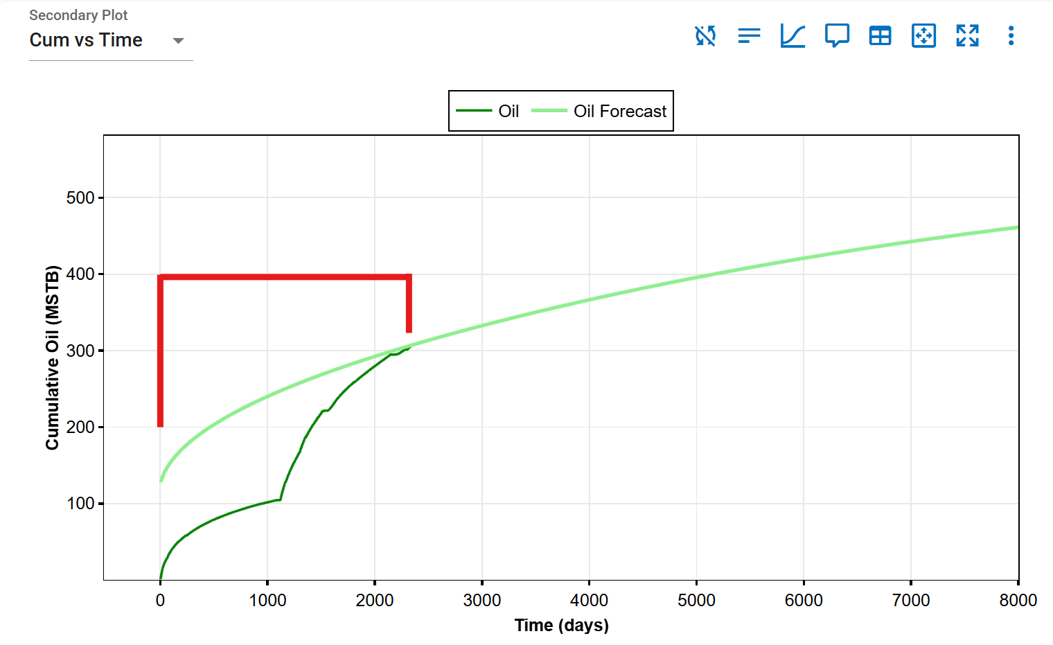
-
Forecast starts before history ends:
References
[2] Pratikno, H., Reese, D.E., Summers, L.E. 2014. Hyperbolic Decline Parameters During and After Linear Flow: Field Example from the Barnett Shale Using Public Data. SPE-171568-MS.