Nodal Analysis - Pressure Gradient Calculator

1. Overview

This feature is used to calculate the fluid properties and approximate the pressure gradient along the well depth. This is very useful to identify high pressure drop sections for erosion, liquid loaded parts of the wellbore along with flow regime classification in the wellbore. This can also used to get infer an approximate depth for gas injection (i.e. depth at which the valve is open for injection gas) by watching the change in pressure gradient across the TVD.

2. Pressure gradient calculations in whitson⁺

Step 1: Navigate to the Nodal Analysis feature and click on the Gradient tab. You will see a default case, populated already with the relevant data for the last date of production.
Step 2: Add cases by clicking the MODIFY CASES button to the top-right of the page, as shown in the GIF below. Click save once done. Each new/edited case runs automatically. You can also rerun the case yourself by clicking the RUN button next to each case.
Step 3: Choose a liquid loading correlation to plot for the critical velocity and critical rates vs depth plot.
Step 4: Generated gradient curves and liquid loading plots should now be available below the case inputs.

3. Technical Features

3.1 Calculated Plots

Here are the main plots generated by this feature:

Pressure or temperature vs TVD or MD of the well - useful for identifying pressure gradient at different sections of the wellbore.
$\label{PressureTempVsMDTVD}$
Superficial gas and critical gas velocity or rates from a correlation of your choice (Turner, Coleman, Nagoo, and Belfroid) vs the TVD or MD of the well - useful for identifying the liquid levels, parts of the wellbore that are liquid loaded.
$\label{VeloRateVsMDTVD}$

3.2 Inputs

This takes into account the following inputs, which can be adjusted by clicking the MODIFY CASES button and using the case input dialog box to edit the cases individually:

Oil, gas and water rates along with any gas injection rates for gas lift and liquid levels for rod pumps.
Tubing head pressure, casing head pressure and any gauge pressures if available (especially for ESP intake).
BHP correlation used to compute the bottomhole pressure.
All of this information can be populated quickly by clicking the calendar icon in the case inputs - directly pick a day in production history to load all the input data required to generate the gradient curves for that day. You can also edit this information in directly in the case inputs (such as adjusting the wellhead pressures for a what-if analysis).

$\label{AddingCasesSimple}$
Current or added wellbore configuration - You can add additional wellbore configurations to test the effects of tubing depth, sizing and different artificial lift for the same production date.
$\label{AddingCasesNewConfig}$

3.3 Outputs

Apart from the main plots generated from setting up the cases, this feature can output the following information in tabular form for every 10 feet of measured depth:

The pressure and temperature.
Superficial gas, liquid and mixture velocities and rates and all critical rate and critical velocity correlation results.
Oil, Gas, Water, Liquid and Mixture densities and viscosities.
Interfacial tension: Oil-gas, water-gas, liquid-gas.
Two-phase flow regimes in the pipe.

You can access this table by clicking the 'extended gradient results' button in the same row as the case, available to the right, for each case.

4. Choke

The choke setting represents a pressure restriction point in the wellbore or surface facility and determines the pressure drop between two points in the system. This is typically between the wellhead and surface flowline, or at a specified downhole depth. Each wellbore configuration includes one choke settings such as choke coefficient, choke depth, and choke size.

What is Choke Coefficient?

The Choke Coefficient is a correction factor used to account for vena contracta effects and irreversible energy losses. This coefficient can be estimated using single-phase valve coefficients provided in manufacturer datasheets, or more accurately determined through field calibration with measured field data.

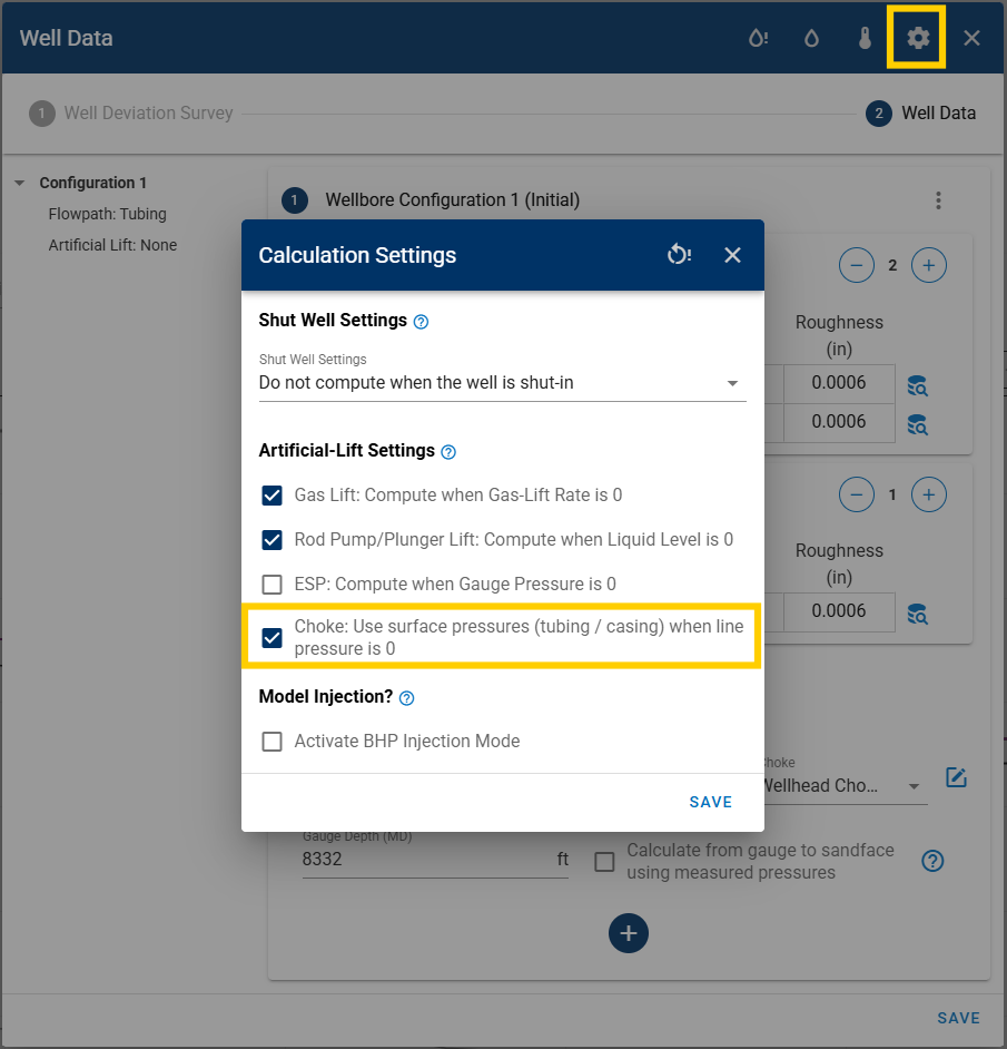
When configuring a choke in whitson⁺, it is important to understand which pressure reference is required depending on where the choke is located:

$\label{choke}$

For wellhead chokes, the line pressure should be used. Otherwise, you can choose to fall back on tubing or casing pressure using the toggle shown below. Moreover, note that the choke depth is always zero and the choke size is fetched from production data.
For Downhole Choke, the default tubing or casing pressure is used. The choke depth and size (opening) are required. If choke size changes with time, user can add new configurations and edit the size for those configurations.

$\label{choke-setting}$

Operational Envelope

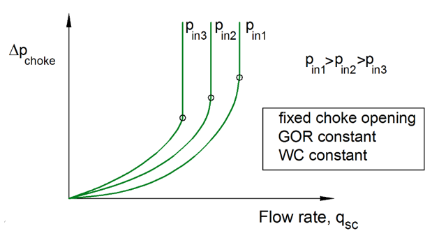
A fixed opening wellhead or bottom-hole choke will display the performance curve (pressure drop vs. surface oil or gas rate), shown in the figure below.

$\label{choke-fix-opening}$

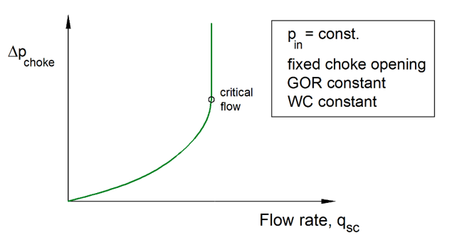
This curve is generated by keeping the inlet pressure, GOR, and WC constant, while changing the downstream pressure from the inlet pressure value to atmospheric conditions (see the sequence plotted in the animation below).

$\label{choke-animation}$

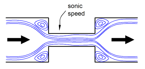
The pressure drop across the choke increases in a non – linear manner when the rate is increased. However, there is a point where it is not possible to increase the rate further (i.e., the pressure downstream the choke does not impact the rate flowing through the choke). This is because the fluid velocity at the throat of the choke has reached the sonic velocity. This typically occurs when the pressure ratio is between 0.5-0.6.

$\label{choke-sonic-velocity}$

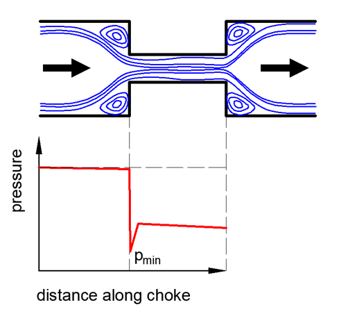
The figure below shows the behavior of pressure along the axis of a bean choke. Note that pressure drops suddenly when the flow encounters the contraction point. In gas-dominated flows this sudden pressure reduction can cause cooling (due to the Joule-Thomson effect), liquid condensation and ice formation (in the presence of free water).

$\label{choke-sudden-drop}$

The figure below shows the performance curve of the choke when the inlet pressure is varied. The pressure drop at which the critical flow is reached increases proportionally with the inlet pressure: $\Delta\, p_c \approx p_{in}-0.5\, p_{in}= 0.5\, p_{in}$ . Changes in GOR and WC give a similar variation of the performance curve.

$\label{choke-vary-inlet}$

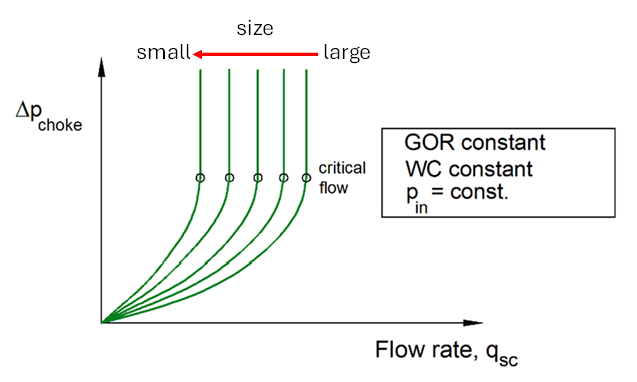
The figure below shows the choke performance curve for 5 different choke openings. A smaller opening will provide a larger pressure drop than a larger opening, and critical flow will be reached at lower flow rates.

$\label{choke-adjsutable-curve}$

Choke Planning Using Nodal Analysis

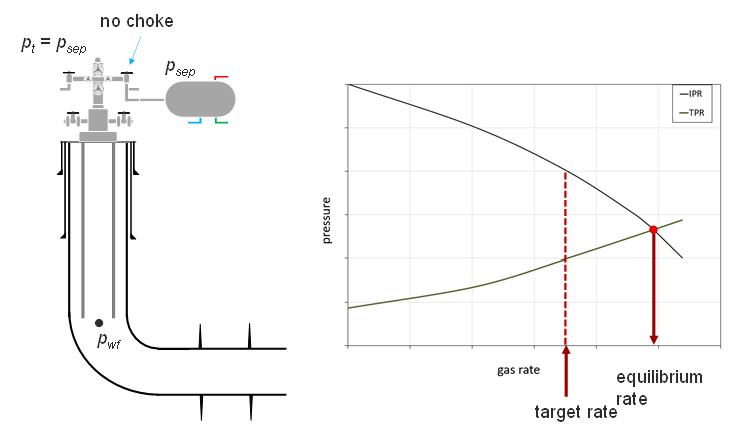
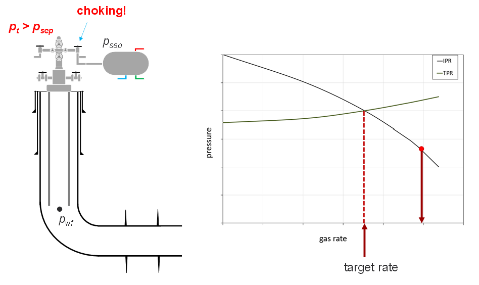
Consider the situation shown in the figure below. A nodal analysis is performed at the bottomhole on a well with no wellhead choke. The equilibrium rate is higher than the target rate; therefore, choking is required.

$\label{choke-nodal-equilibrium}$

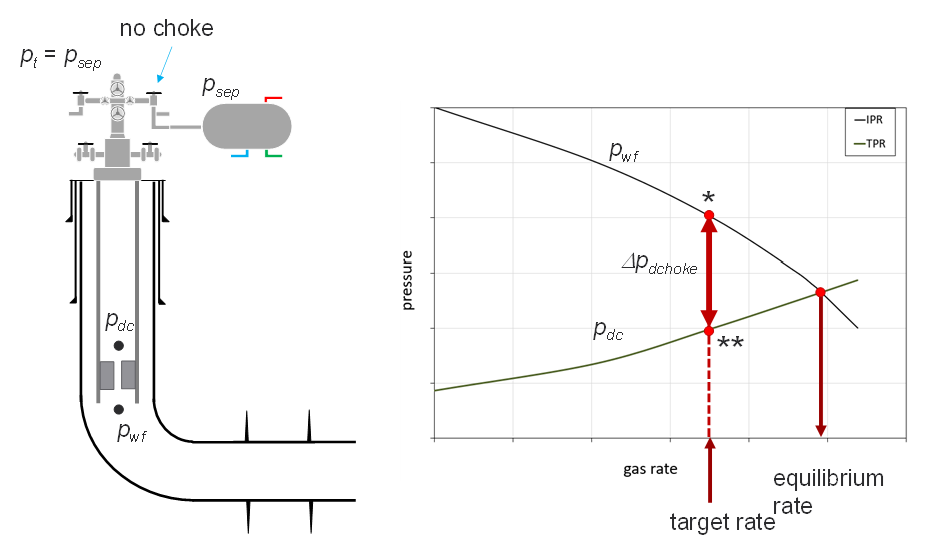
If a bottom-hole choke is used, the choke must drop the pressure from the pressure available from the reservoir (marked with * in the figure) to the pressure required to flow to the surface through the tubing (marked with ** in the figure).

$\label{choke-nodal-equilibrium-2}$

Another alternative is to use wellhead choking (shown in the figure below). In this approach, wellhead choking increases the tubing head pressure and “shifts” the TPR up, moving the intersection to the left.

$\label{choke-nodal-equilibrium-3}$

Choke Modeling

Chokes are often modeled by integrating the differential version of the momentum equation between the choke inlet and the throat and assuming no friction or localized losses between these two points. Due to the convergence of the flow, the effective throat cross-section area (often referred to as vena contracta) is not exactly equal to the throat cross-section area ( $A_{\text{throat}}$ ), thus a correction factor ( $C$ ) is introduced ( $A_{\text{throat,effective}} = A_{\text{throat}} \cdot C$ ) and is often varied in the range (0,1] such that the model predicts accurately measured data.

The one-dimensional momentum equation in differential form for liquid-gas flow, neglecting friction and localized losses, is:

$\begin{equation} -\, \mathrm{d}p\, =\, H_l\, \rho_{g}\, V_g\, \mathrm{d}V_g\ +\, H_g\, \rho_l\, V_l\, \mathrm{d}V_l\ \end{equation}$

where $H$ is holdup, $V$ is velocity, $\rho$ is density, and $p$ pressure.

The whitson⁺ model assumes liquid and gas travel at the same velocity (mixture velocity, $V_m$ , equal to the sum of local rates of oil, gas and water divided by cross-section area). Then, the equation above is integrated between the inlet and the throat, while neglecting inlet velocity, to obtain:

$\begin{equation} -\, \int_{p_{\text{inlet}}}^{p_{\text{throat}}} \frac{1}{\rho_{m, \text{homogeneous}}}\, \mathrm{d}p\, =\, \frac{\left(V_{m, \text{throat}}\right)^2}{2} \end{equation}$

$\rho_{m, \text{homogeneous}}$ is the homogeneous mixture density, defined as:

$\begin{equation} \rho_m =\, \frac{1}{\frac{x}{\rho_g} + \frac{\left(1-x\right)}{\rho_l}} \end{equation}$

where $x$ is the gas mass fraction, and $\rho_g$ , $\rho_l$ are the gas and liquid phase densities, respectively.

Calculation Details

In all whitson⁺ applications like bhp calculations and nodal analysis, rate across and pressure downstream the choke are known, and it is desirable to find inlet pressure.

The equation is solved by computing numerically the homogeneous density integral, assuming isothermal flow and thermodynamic equilibrium. However, there is some care to be exercised about the pressure value to employ at the throat.

When operating in the subcritical regime, the pressure downstream of the choke is usually employed to approximate the pressure at the throat, assuming there is very little pressure recovery after the throat. When operating in the critical regime, the pressure measured downstream of the choke is lower than the pressure at the throat and is initially unknown. The main challenge is that often it is not known beforehand if the choke is operating in the critical or subcritical regime, so the calculation requires some trial and error.

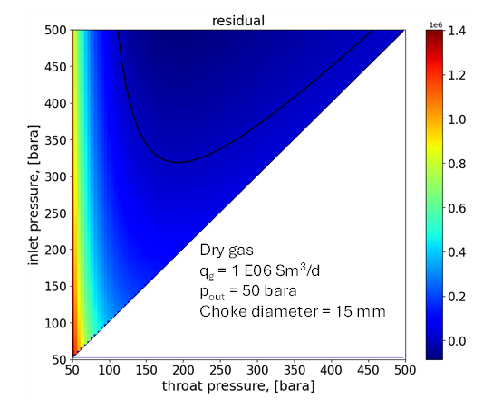
As an example, consider the flow of dry gas through a choke, outlet pressure equal to 50 bara, inlet temperature 80 °C. The figure below shows the value of the residual of the choke model for a rate of 1e6 Sm³/d, and for several combinations of inlet pressure and throat pressure values, from 50 bara to 500 bara. Cases where the inlet pressure is lower than the throat pressure are discarded. The black line is the inlet-throat pressure combinations where the residual is zero (potential solutions to the choke model). The physical solution is the minimum point in the black curve. When the minimum lies when the throat pressure is equal to the downstream pressure, the choke operates in the subcritical regime. Otherwise, the choke operates in the critical regime (like in the figure below).

$\label{choke-model}$

Recommended Practice for BHP Calculations

When estimating BHP, always aim to use the shortest and most reliable pressure path. If there is a wellhead choke, but measured tubing head pressure or casing head pressure is available and considered reliable, it is generally best to ignore the wellhead choke and calculate BHP directly from this surface pressure. Doing so minimizes assumptions, simplifies the pressure path, and improves accuracy.

Preferred Calculation Path:

Tubing/casing head pressure → tubing/casing pressure drop → bottomhole pressure

This direct approach is preferable to the more assumption-heavy path that includes a wellhead choke:

Line pressure → wellhead choke pressure drop → tubing/casing head pressure → tubing/casing pressure drop → bottomhole pressure

This distinction is especially important when high-confidence surface pressure data is available — performing wellhead choke calculations in such cases may unnecessarily introduce uncertainty.

When Downhole Gauge Data Available

If a downhole pressure gauge is available, it is best to use that data directly for BHP estimation. This eliminates the need for pressure gradient assumptions and calculations entirely, resulting in the shortest and more reliable output.

When to Use Wellhead Choke-Based Calculations

Surface pressure is unavailable or unreliable, but line pressure and flow rates are available.
Line pressure and surface pressure are available, but flow rates are unavailable or unreliable (an iterative approach will be used to adjust rates until the calculated surface pressure matches the measured value)
Simulating or designing choke strategies for operational optimization, such as evaluating pressure response or production control, erosion mitigation, etc

5. Example

Here's an example, showing how to add a case simulating an increased gas injection rate and generating extended gradient results vs depth:

$\label{AccessingExtendedGradientResults}$