Type Well
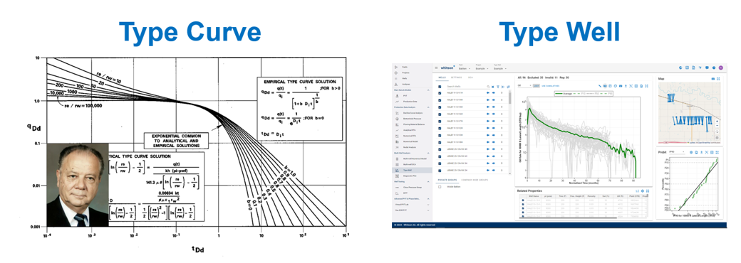
- “Type Wells” are often referred to as “Type Curves.”
- “Type Curves” are idealized production profiles (based on equations and/or numerical simulation) against which actual production results are compared.
- “Type Wells” are based on actual well production data and represent a typical production profile for a collection of wells over a specified duration.
Production rate basis (stock tank rates)
Type Wells are built from stock-tank (standard-condition) rates, either provided directly or converted from separator-rate data using whitson+ when separator conditions vary over time.
What is a 'typical' well?
The arithmetic mean of a group of wells is commonly used as a measure of central tendency and, therefore, to estimate a Type Well. However, experts such as David Fulford argue that the geometric mean may better represent central tendency. Production rates and EURs are generally lognormally distributed; accordingly, averaging their logarithms (i.e., using the geometric mean) makes intuitive sense. Both options are available in whitson+.
1. Create a Type Well Scenario
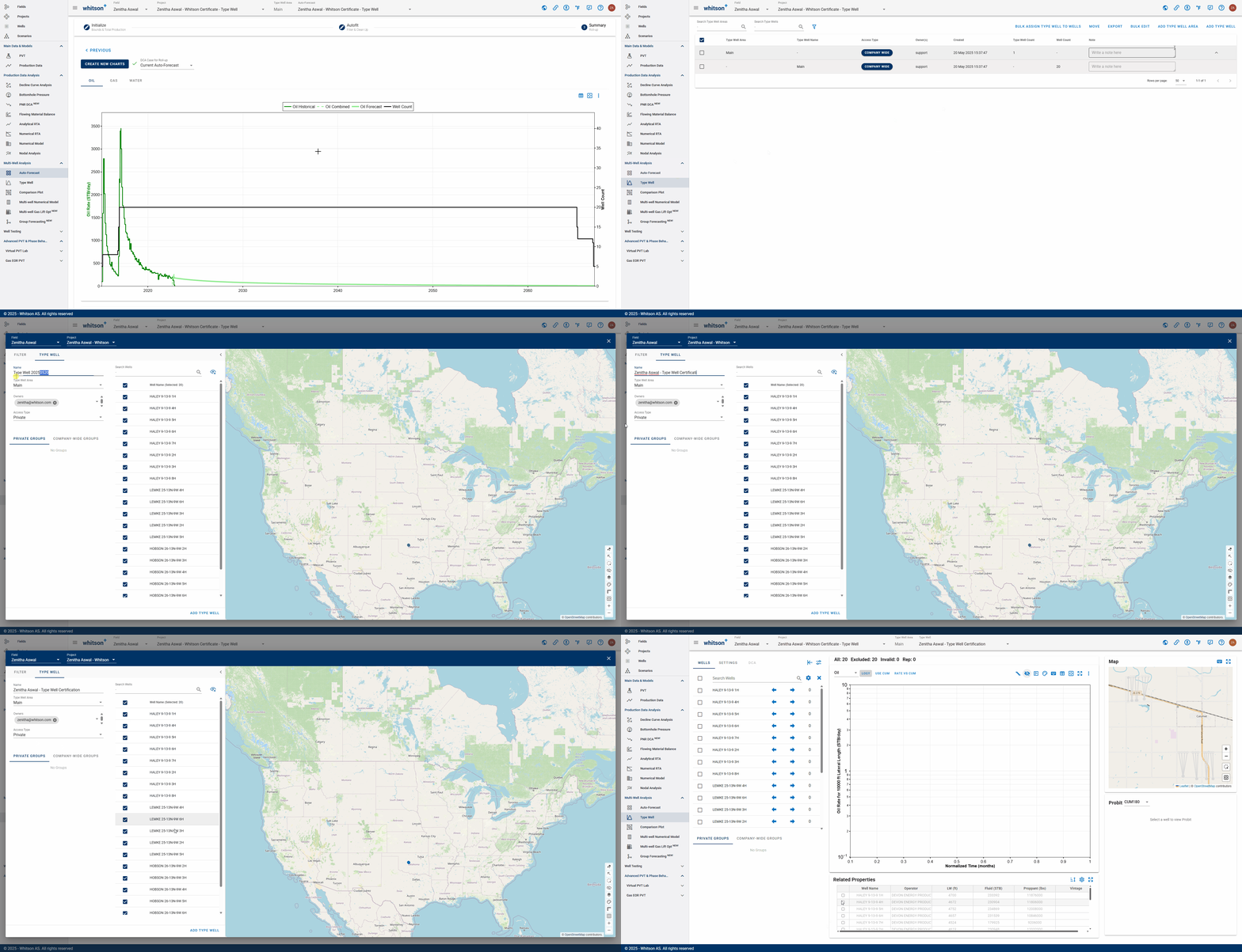
- Click Type Well in the navigation panel (just under Auto-Forecast).
- To the upper right, click ADD TYPE WELL.
- Enter a name for the scenario. Select all wells by clicking the checkbox at the top of the well list (to the left of Well Name), or select individual wells by clicking the checkbox next to each one.
- Click SAVE in the lower-right corner.
You can store multiple Type Wells per project
This page provides an overview of the Type Wells, including when and by whom they were created and which wells were used to create them.
2. Generating a Type Well
2.1. Well Selection
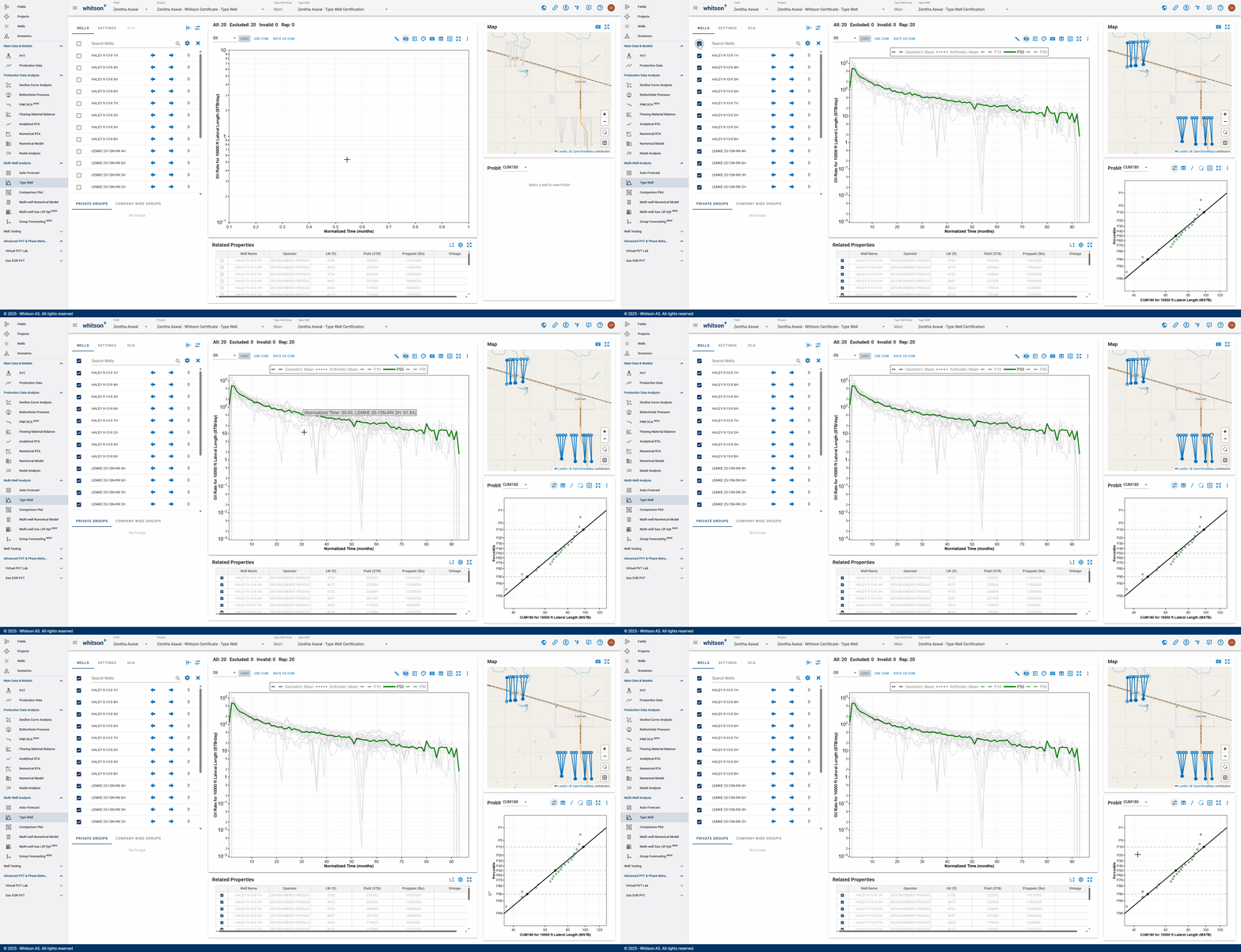
Click the checkbox next to Search Wells to include all wells available in the Type Well scenario.
There are two ways to include or exclude individual wells when creating the Type Well:
- Click the checkmark next to the well name.
- Ctrl-click the time series to exclude that well from the Type Well.
You can also select a well by clicking one of its time-series data points on the graph. This filters the well menu on the left to show only that well. Alternatively, search for the well by name in the Search Wells field.
2.2. Pick Relevant Phase
First, you must pick the phase for which you would like to build a Type Well.
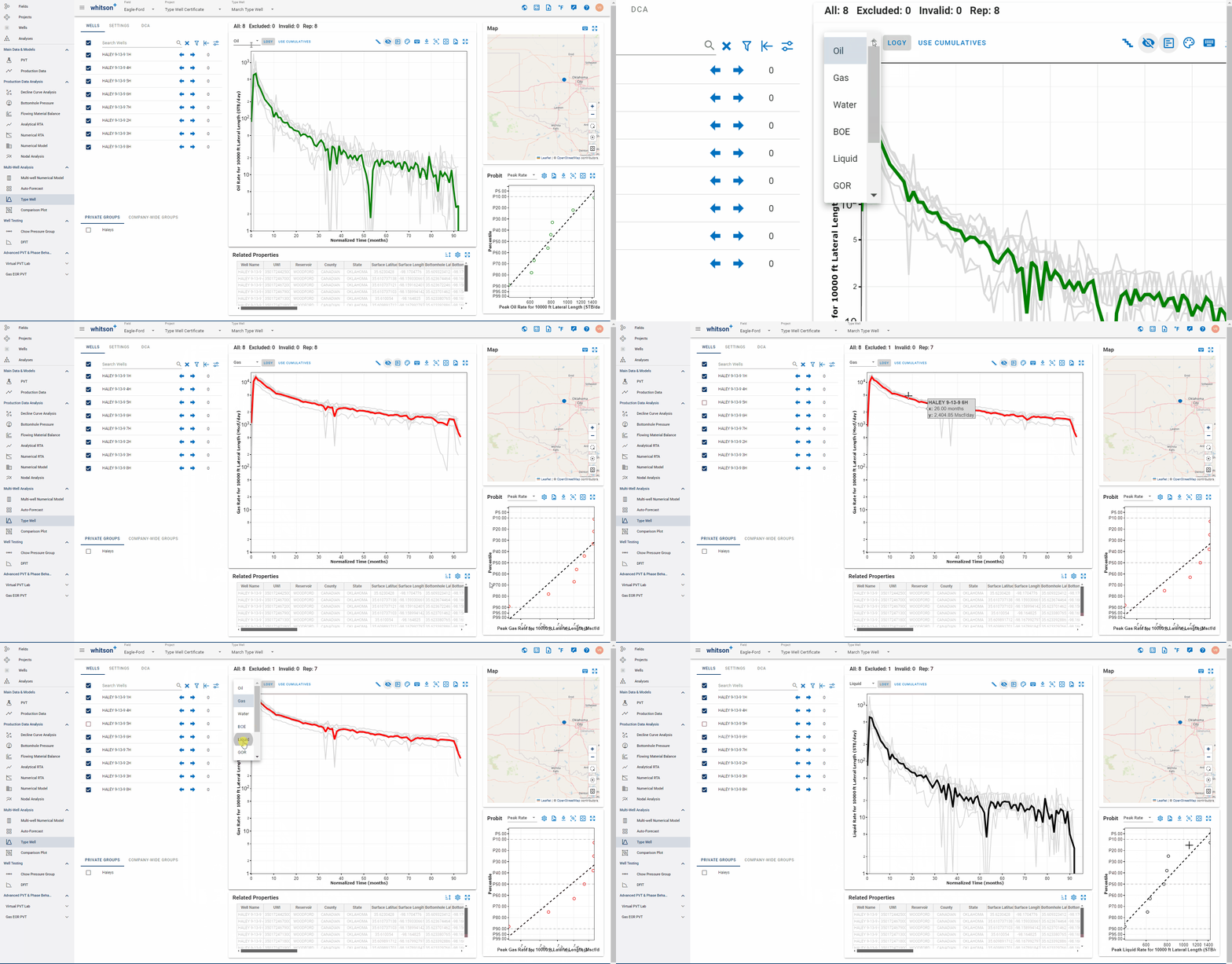
In the Settings tab, you can configure the x-axis and time resolution, select the y-axis normalization parameter and multiplier, switch between averaging methods, and append a previously saved Auto-Forecast or single-well DCA forecast, as described in the sections below.
2.3. Ratio Type Well
To create a ratio Type Well, you must first create and save a Type Well case for the Primary phase (Oil, Gas, or Water).
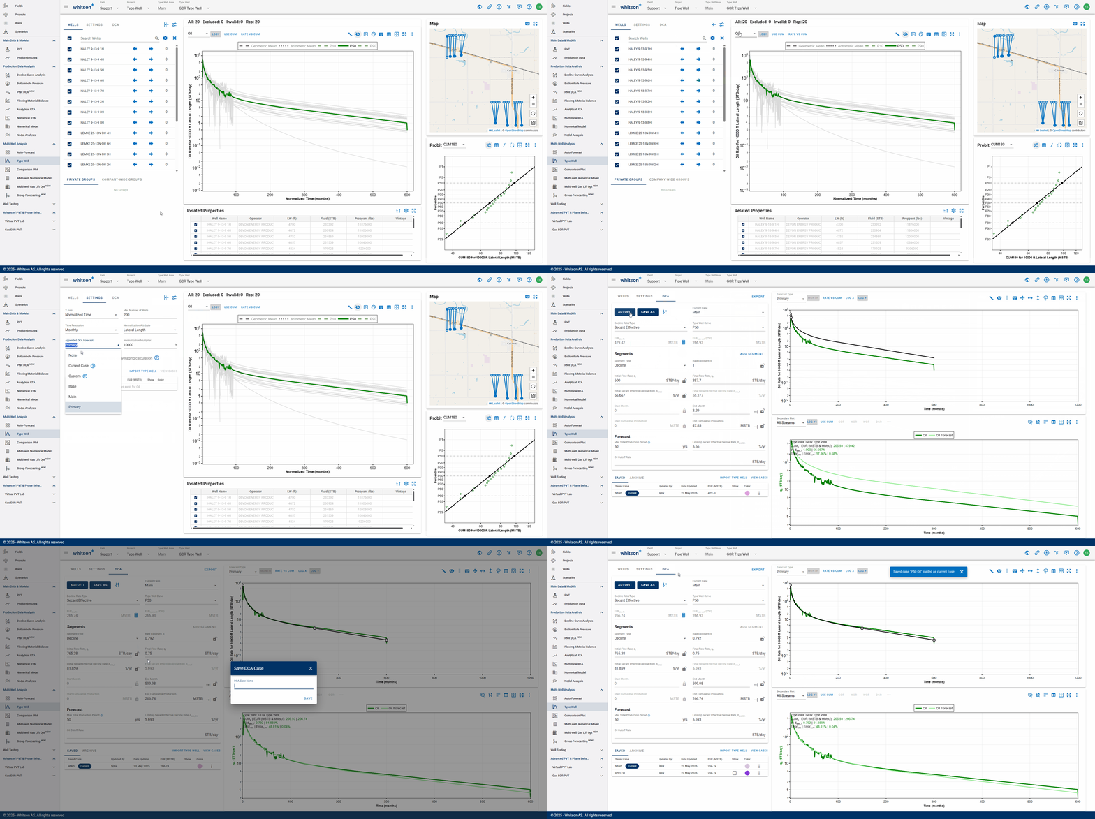
Once the Primary Type Well is saved, switch the phase above the plot (on either the Wells or Settings tab) to the Ratio phase (GOR, WOR, WGR, or OGR). If you have already performed DCA forecasting on a ratio phase, you can append the forecast to the well profile in the plot. In the example below, the GOR forecast case named "Base" is appended to the well.
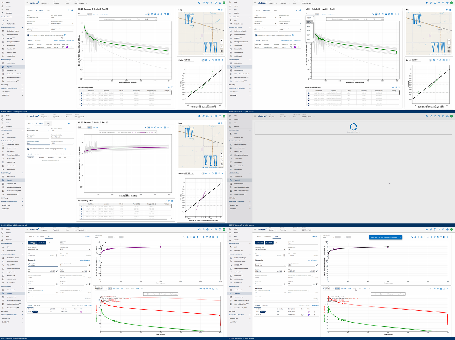
After switching to a Ratio phase, click the DCA tab. The Select Primary Phase window prompts you to select a saved Primary Type Well case. For GOR, the primary phase can be either a saved gas case or a saved oil case. Because we created the "Oil P50" Type Well earlier, we can use it as the primary phase. This action opens the DCA interface, where you can adjust the fit line for the ratio Type Well.
Info
Saving a ratio Type Well also generates a corresponding Type Well for the secondary phase. In this example, the saved GOR Type Well created from the Primary Oil Type Well is also listed under the Gas phase and can be plotted as the Gas Type Well.
3. Overview of Plot Options
Watch the video above for an overview of the plot options. The icons in the upper-right corner of the plot are summarized below:
- Show/Hide Well Count: Use the stairs icon to show or hide the number of wells over time.
- Show/Hide Individual Well Production Data: Click the eye icon to show or hide individual well production data (in gray).
- Show/Hide Legend: Use the legend to display the P90, P50, and P10 curves, which are hidden by default.
- Downloads: Export the Type Well data, including the individual well rates displayed on the plot, to an Excel spreadsheet. You can also export the current plot as an image as an png or svg or a PowerPoint presentation. There is also an option to copy the iage to the clipboard for easy access to plot outside of whitson+.
- Zoom Options: Use the standard controls to zoom in or out.
3.1. Plot Colors
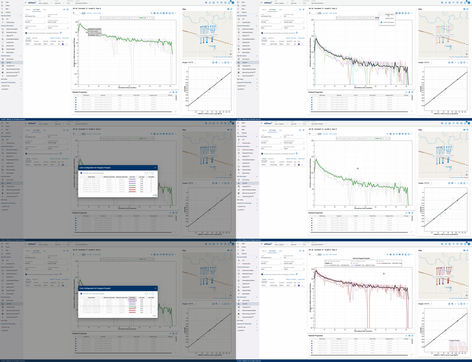
Use the color palette icon to spread colors, color by attribute (such as well data, reservoir properties, or completion metrics), or restore the default colors, as shown in the GIF below.
Pro tip
You can also copy and paste colors from one box to another. This technique works in Comparison Plots and anywhere else colors can be adjusted manually in whitson+.
3.2. Nice-to-know items
3.2.1. Time Align
Additionally, in the well selection pane on the left, you have options to:
- Start at peak time: Constructs the Type Well from the peak rate by moving each well's peak rate to time = 0.
- Start all plots from time = 0: Constructs the Type Well by aligning each well's first production with time = 0.
Time Alignment
Time Align on First Production
- Strength: For larger well sets, represents the production profile while accounting for time to peak.
- Weakness: may not accurately reflect production decline behavior.
Time Align on Peak Rate Date
- Strength: More accurately reflects production behavior.
- Weakness: Excludes ramp-up time, which may have a small impact on EUR but is important for first-year revenue projections.
- Bulk Shift Wells: Shifts all wells by the specified number of days. Negative values shift left, positive values shift right. Two types of Shift Mode is available:
- Replace all existing shifts with this value: Replaces the current shift for all selected wells with the specified value. Any previously applied shift is overwritten. For example, entering 5 sets the shift for every selected well to 5 days, regardless of its previous shift value.
- Increment/decrement existing shifts: Adjusts the current shift for all selected wells by the specified value. Positive values increase the existing shift, while negative values decrease it. Wells with no existing shift are treated as having a shift of 0 days before the adjustment is applied.
- Aligns Peak: Constructs the Type Well by aligning each well's peak rate.
- Search and filter wells: Filters are applied across the software, so filters applied elsewhere also appear here, and vice versa.
- The X icon clears the search bar.
- You can also use the arrow buttons next to a well name to shift that well's production data left or right in time.
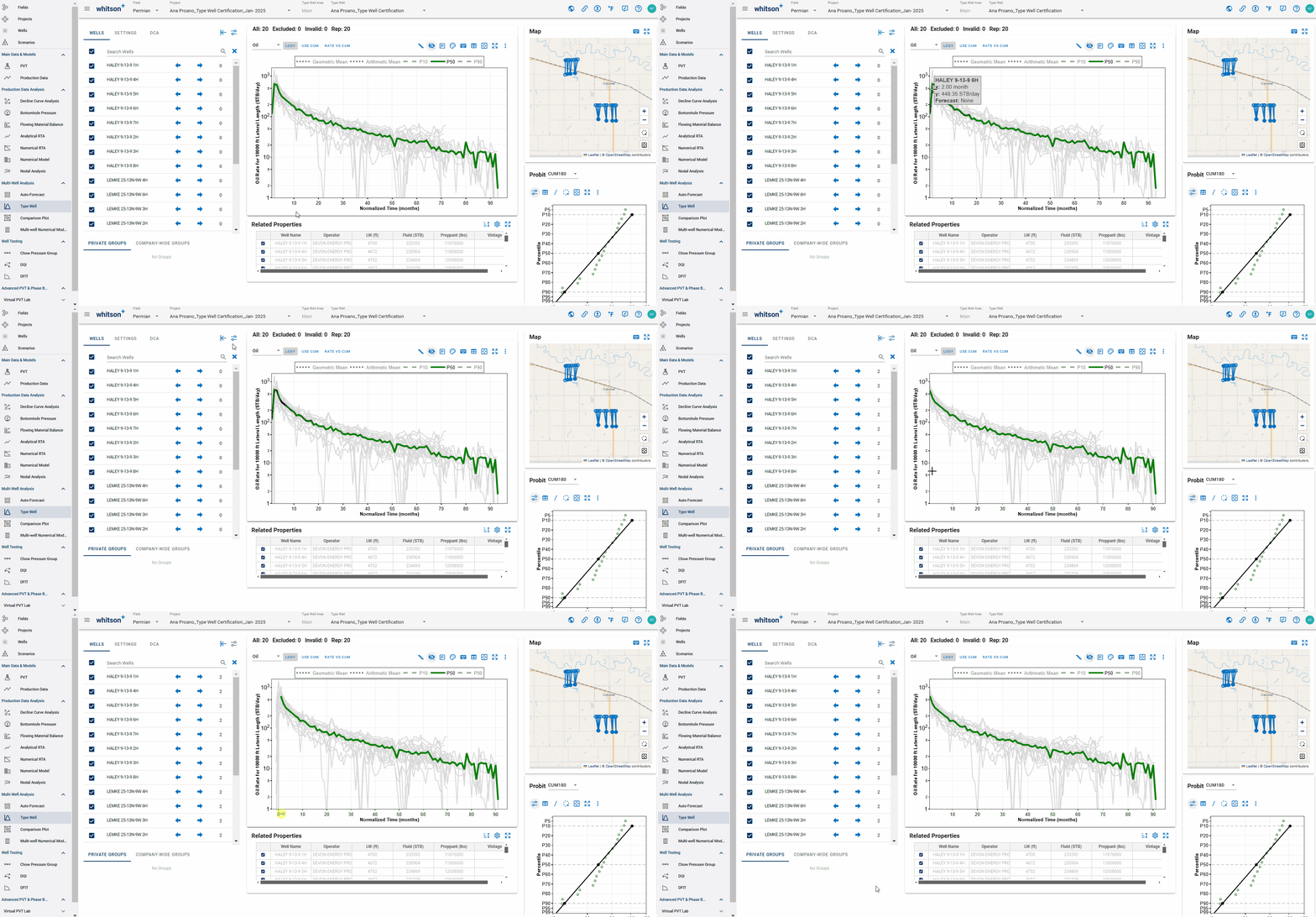
3.2.2. Manage Templates
Most Type Well settings can be saved as a template and reused across different Type Well projects. Templates help maintain consistent settings between projects while reducing the time required to configure each Type Well individually.
3.2.2.1. Creating a Template
After configuring the Type Well settings, click the Manage Template icon shown below.
Enter a name for the template and click CREATE. The template will be saved and made available for future use.

3.2.2.2. Applying a Template
Templates can be applied in two ways:
- Individual Type Well Project: Open the desired Type Well project, click Manage Templates, and select the template you want to apply. The saved settings will be applied automatically to the current Type Well project.

- Multiple Type Well Projects: From the Type Well module, click ACTIONS in the upper-right corner and select Bulk Edit. Choose Apply Template, then select the desired template from the dialog box and hit APPLY. The selected template will be applied to all selected Type Well projects.

3.2.3. Highlighting Individual Wells Across All Plots
There are several ways to highlight wells across all the plots:
- Click a well name in the well list to highlight the well in yellow across all plots. This allows you to compare it with the Type Well, identify its location on the map, and see its relative ranking in the probit plot.
- Click a time-series data point on the graph. This automatically filters the well list to show the relevant well, which is then highlighted in yellow across all plots.
- The Probit plot has the option to use a lasso highlight to select the data points (wells) of interest. These selected wells will then be highlighted in yellow in the type curve plot and the map.
- The map also allows you to use a lasso highlight to select the well locations of interest. These selected wells will then be highlighted in yellow on both the type curve plot and the probit plot.
Filtered Wells and Map Legend
The Type Well map includes additional controls for reviewing filtered wells:
- Use the eye icon to show or hide wells that have been filtered out.
- The map legend uses the configured colors to identify the corresponding well groups/ranges.
These options are shown in the GIF below:
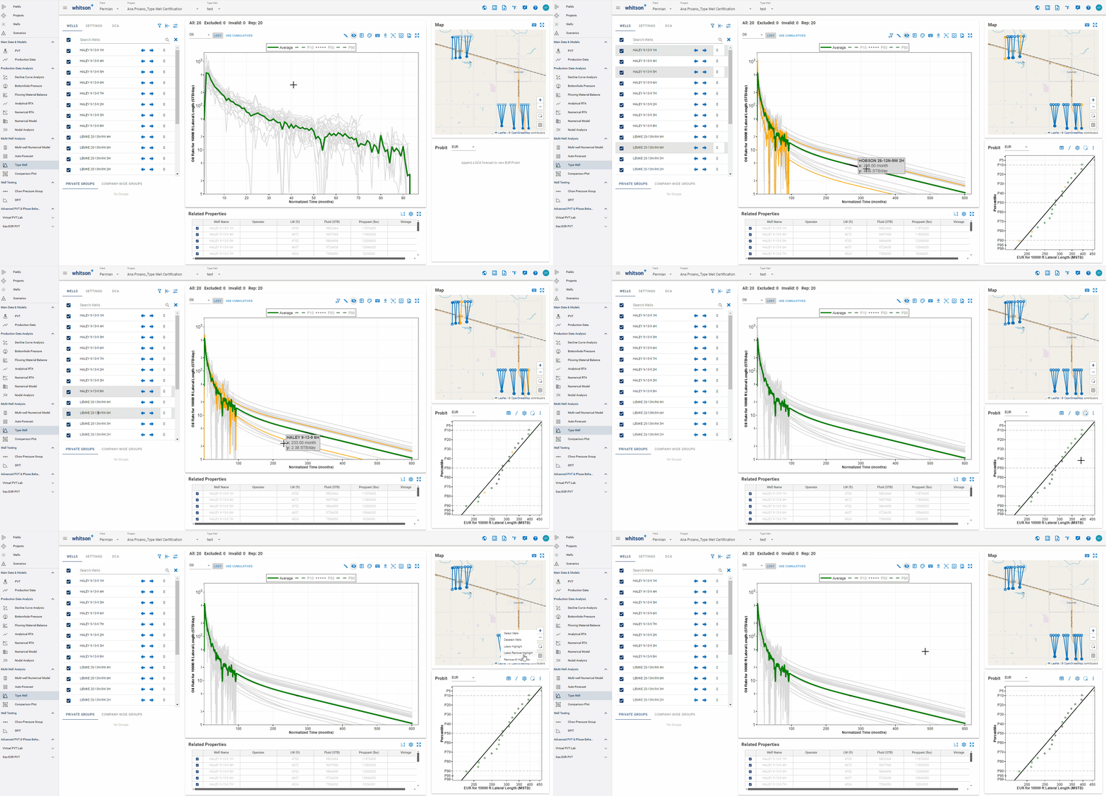
To remove the highlighted wells, click the 'Remove all highlights' icon.
Well Count Status Definition
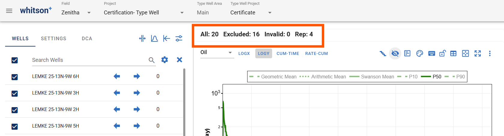
- All: Total number of wells selected in the entire Type Well project.
- Excluded: Wells that are currently not selected.
- Invalid: A well is marked as invalid if any of the following conditions are true:
- The well does not have production data.
- The well is missing the required normalization property (for example, normalization is based on lateral length, but the well does not have a lateral-length value).
- The well exceeds the “Max Number of Wells” limit set for the Type Well.
- Rep: Short for Representative. This indicates the number of wells that are currently selected and plotted.
3.3. Probit Plot
Append DCA Forecast
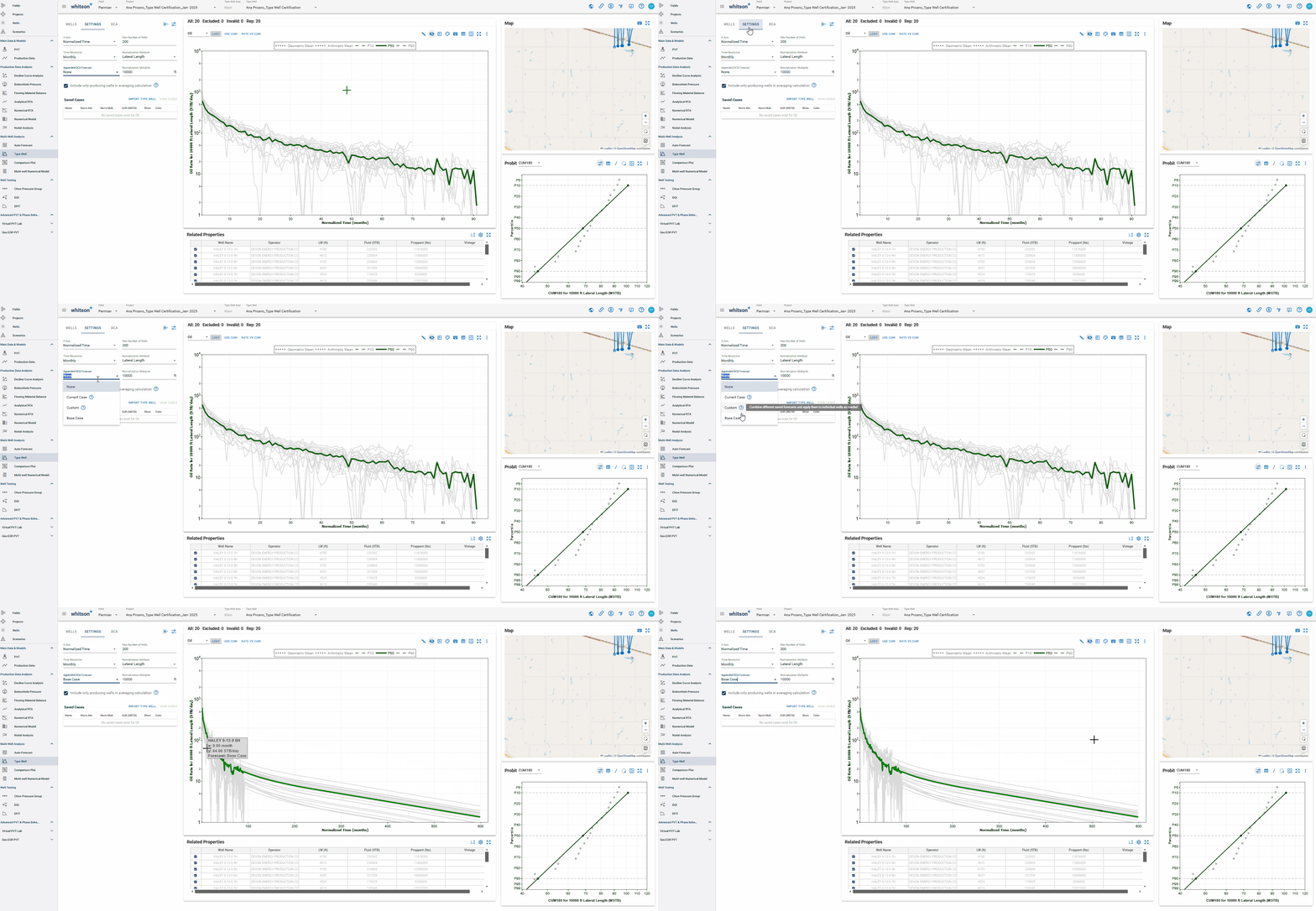
Appending the forecast as shown in the GIF above populates the probit plot.
Probit Plot
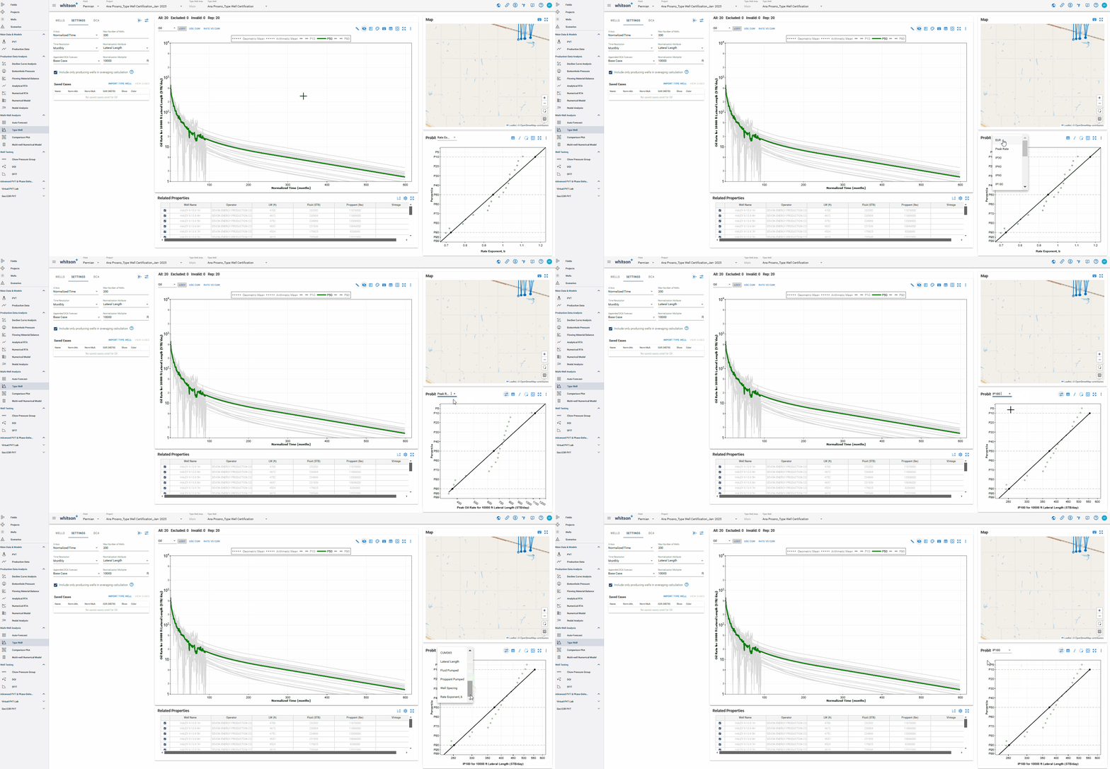
- Represents the statistical distribution of a metric (e.g., EUR, IP60, or a physical parameter) at a selected point in time.
- The shape can help determine whether the results follow a lognormal distribution.
- A “probit best-fit” regression can provide statistical insights, including a measure of uncertainty (e.g., the P10/P90 ratio).
Additional Probit functionality
- EUR/ft: display EUR normalized by lateral length as an available Probit metric.
- UWI hover information: hover over a Probit point to view the corresponding UWI.
- Single-click highlighting: click an individual Probit point to highlight the corresponding well across the Type Well plots and map.
4. Probabilistics
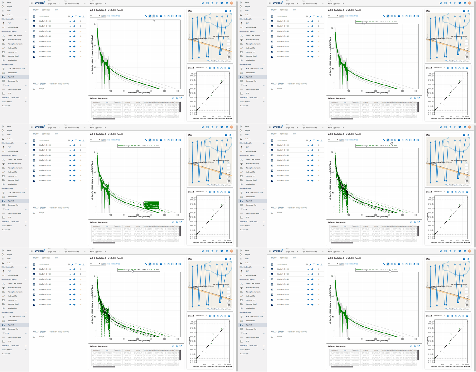
The P10, P50 and P90 time series are not shown by default. Add them by clicking on the legend. You can also choose to display the Well Name and/or UWI as shown above.
5. Settings
5.1. Max Number of Wells
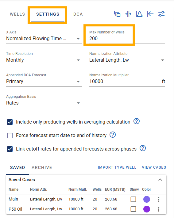
While there's no technical limit, processing time can be impacted by the number of wells. The default is 200 wells; adjust this setting if you need to process a larger number of wells.
5.2. X-Axis Normalization
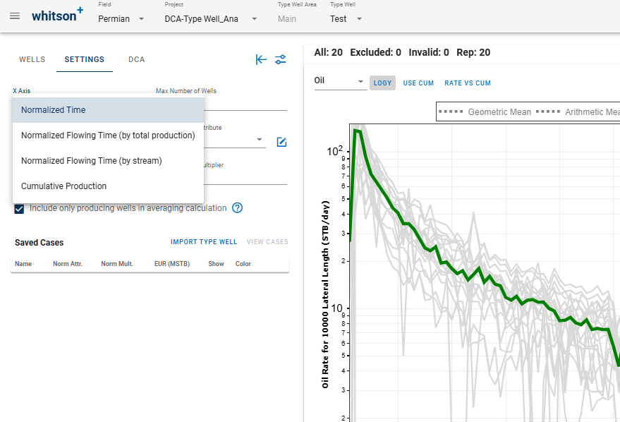
There are four different x-axis time options available:
- Normalized Flowing Time (by stream): Includes only time steps when the rate of the selected stream (oil, gas, or water) is nonzero.
- Normalized Flowing Time (by total production): Includes only time steps with active oil, gas, or water production and excludes periods when all rates are zero.
- Normalized Time: Aligns time with first production.
- Cumulative Production: Plots cumulative production on the x-axis.
5.3. Time Resolution
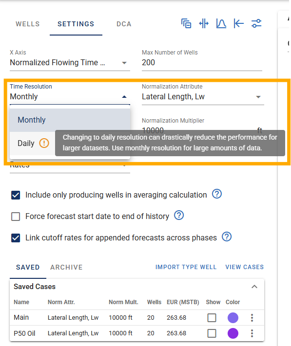
You can choose between monthly and daily resolution.
-
Monthly: The default resolution, recommended for large datasets.
-
Daily: Provides more detailed results but can significantly affect performance, especially with larger datasets.
5.4. Y-Axis Normalization (Normalization Attribute)
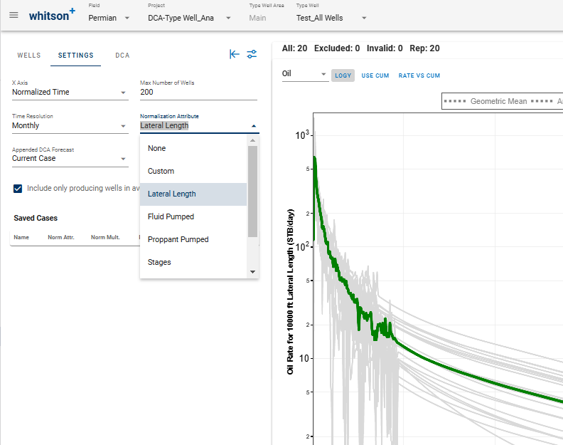
Use dimensional normalization to choose either the unnormalized rate or a rate normalized by a property such as lateral length, fluid pumped, proppant pumped, stages, clusters, number of fractures, or a custom attribute. Normalization standardizes the data and places the wells in a meaningful comparative context.
5.5. Lateral Length + Peak Rate Normalization
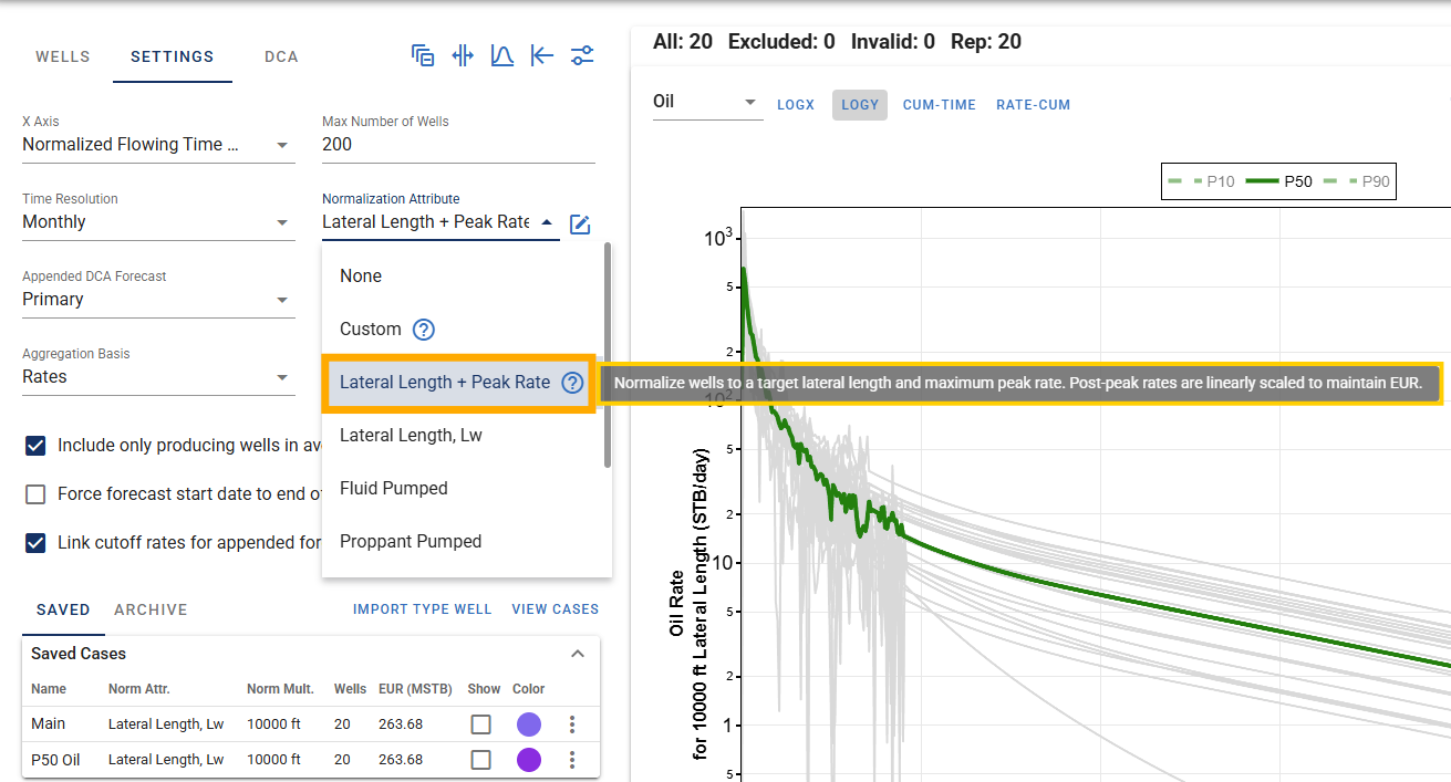
First, each well is linearly scaled to the target lateral length. If a peak-rate constraint is applied, production is capped at that rate, which reduces early-time volumes. To keep total recovery unchanged, the volume lost because of the cap is recovered later by uniformly scaling the production profile from the peak onward. For each well, a single linear scaling factor is calculated so that all post-peak rates are increased proportionally and the final EUR matches the EUR obtained before the peak constraint was applied.
The post-peak scaling is calculated using a goal-seek approach. The algorithm iteratively adjusts a single global multiplier and recalculates cumulative production while capping early-time rates at the peak. It continues until the total recovered volume matches the laterally scaled EUR calculated before the peak constraint was applied.
5.6. Normalization Multiplier
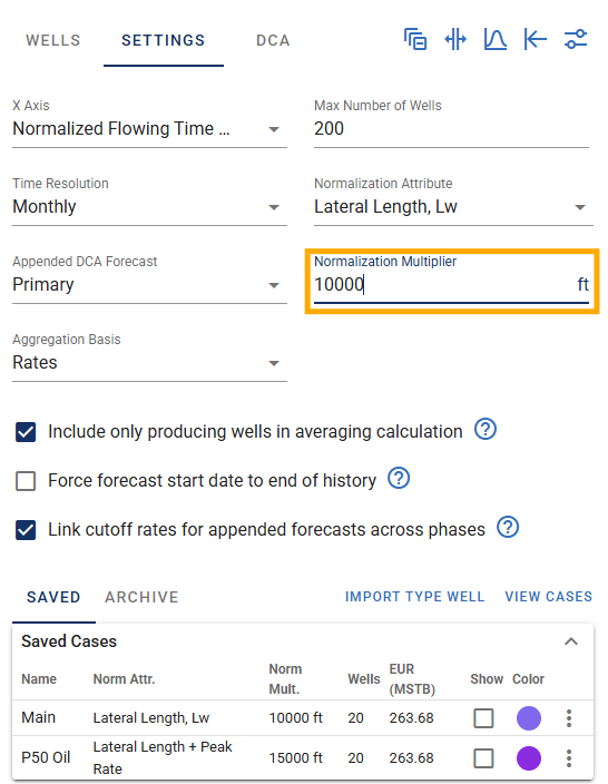
You can also use the normalization multiplier to convert the normalized rates to a likely actual rate for a presumed value of the normalization variable (e.g., 10,000 ft lateral length).
5.7. Append DCA Forecast
Append a previously saved DCA forecast to each well's historical data. Beyond the historical period, the resulting Type Well is the average of the individual forecasts—i.e., it represents “averaging the forecasts.”
You can select from the following options:
- None: Do not append a DCA forecast.
- Current Case: This is the DCA case currently applied to the well.
- Saved cases from the Auto-Forecast module.
- Saved cases from the Single-Well DCA module.
Append the forecast as shown in the GIF above.
Pro tip
If you prefer not to use Auto-Forecast, save each individual well's decline-curve forecast under the same name. That name then functions like a saved Auto-Forecast case; selecting it from this dropdown adds the forecasts for all wells.
5.8. Aggregation Basis
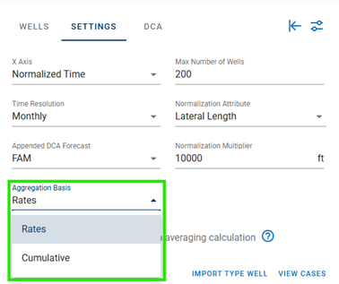
The Aggregation Basis lets you choose how probability declines (P10, P50, P90, Geometric Mean, Arithmetic Mean, Swanson Mean) are calculated. You can base the calculation on either:
-
Rate – Aggregates the probability decline using the production rate at each timestep.
-
Cumulative Production – Aggregates based on the total production accumulated up to each timestep.
This flexibility allows you to analyze well performance in the way that best fits your workflow and reporting needs.
5.9. Auto-Calculated Ratio Type Wells
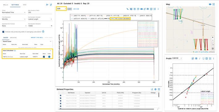
Auto-Calculated Ratio Type Wells streamline the creation of ratio-based Type Wells (e.g., GOR, OGR, WGR) by eliminating the need for manual curve fitting.
When multiple Type Wells with the same case name exist within the same project (for example, a gas and an oil Type Well both named TWP X), the software automatically combines them to generate the corresponding derived ratio Type Wells.
Key characteristics:
- No manual decline or ratio fitting is required
- Ratio curves are calculated directly from the underlying Type Wells
- Ensures consistency between rate-based and ratio-based Type Wells
- Significantly accelerates multi-fluid Type Well construction and analysis
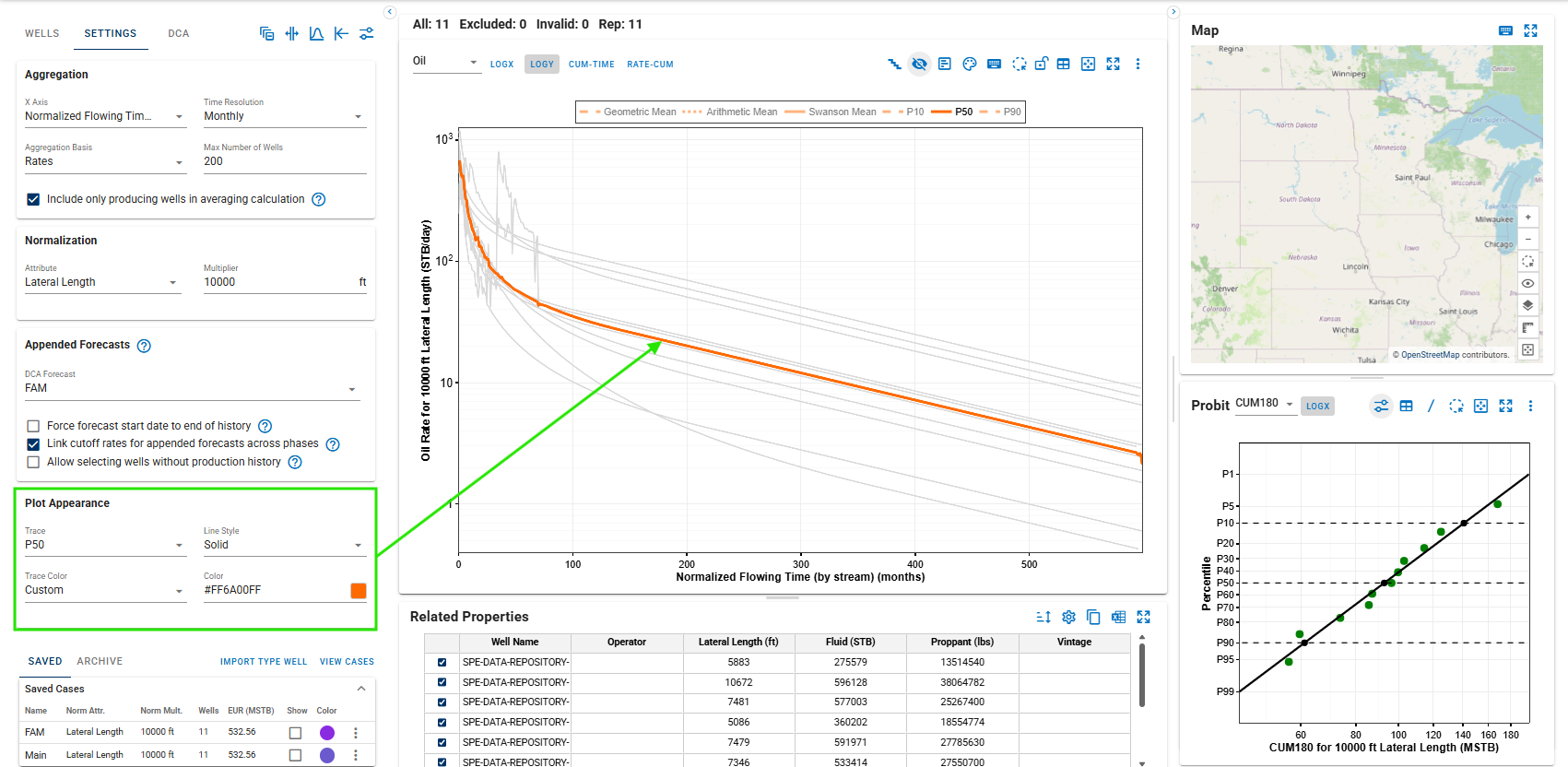
5.10. Individual Trace Style and Color
Individual well traces can be customized independently using Trace Style and Trace Color.
- Trace Style: changes the line style used for the selected trace.
- Trace Color: changes the color assigned to the selected trace.
These settings make it easier to distinguish selected analog wells or other traces from the full Type Well population.
5.10. Hotkeys
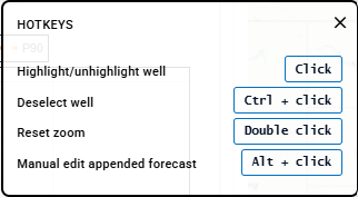
- After a DCA forecast has been appended to the Type Well workflow, hold Alt and click the appended forecast on the plot to open it for editing.
6. DCA: Forecast the Average vs. Average the Forecasts
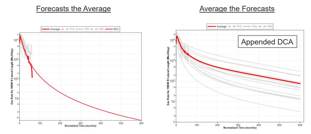
You can either Average the Forecasts or Forecast the Average.
What's the difference?
Average the Forecasts
- Time-consuming without the Auto-Forecast option.
-
Useful for statistical evaluation and P10/P90 quantification of EUR.
➜ Use the Append DCA Forecast dropdown on the Settings tab.
Forecast the Average
- Apply a decline to the truncated Type Well to obtain a full-life production profile and EUR.
-
This approach is time-efficient but does not provide a distribution of EURs.
➜ Use the DCA tab in the Type Well.
In this section, we'll forecast the Type Well (average) and the P90, P50, and P10 curves using DCA. You can also force the DCA fit to honor the EUR of the Type Well by enabling Set EURType Well = EURDCA fit. You can save this DCA fit to the Type Well or to a P90, P50, or P10 curve. Enable the saved fit on the Settings tab to display it on the main Type Well plot, as shown in the GIF below.

6.1. Cumulative Calculation in Type Well vs DCA
When constructing a type well, we need to build a curve all the way from time 0 to the end of the historical data. If a DCA forecast is appended, the type well constructed beyond historical data will be the average of the forecasts — i.e. 'averaging the forecast'.
This approach differs from DCA/PDP forecasting, which primarily focuses on the period from the end of the historical data forward, although the fit may begin at the peak rate.
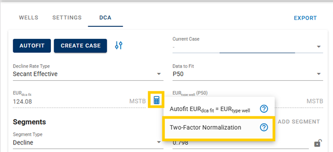
6.2. Two-Factor Normalization in DCA
This method independently adjusts the peak rate and EUR to achieve nonlinear scaling. The peak rate is scaled directly using a multiplier, while the decline rate is calculated to deliver the target EUR.
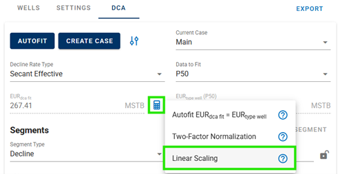
6.3. Linear Scaling in DCA
Linear scaling applies a constant factor to all segments, modifying the initial (qi) and final (qf) rates in the DCA segment fit without changing the decline-curve shape.
7. P10, P50, and P90: Percentile Lines vs. Probit Plot
7.1. Probit Plot
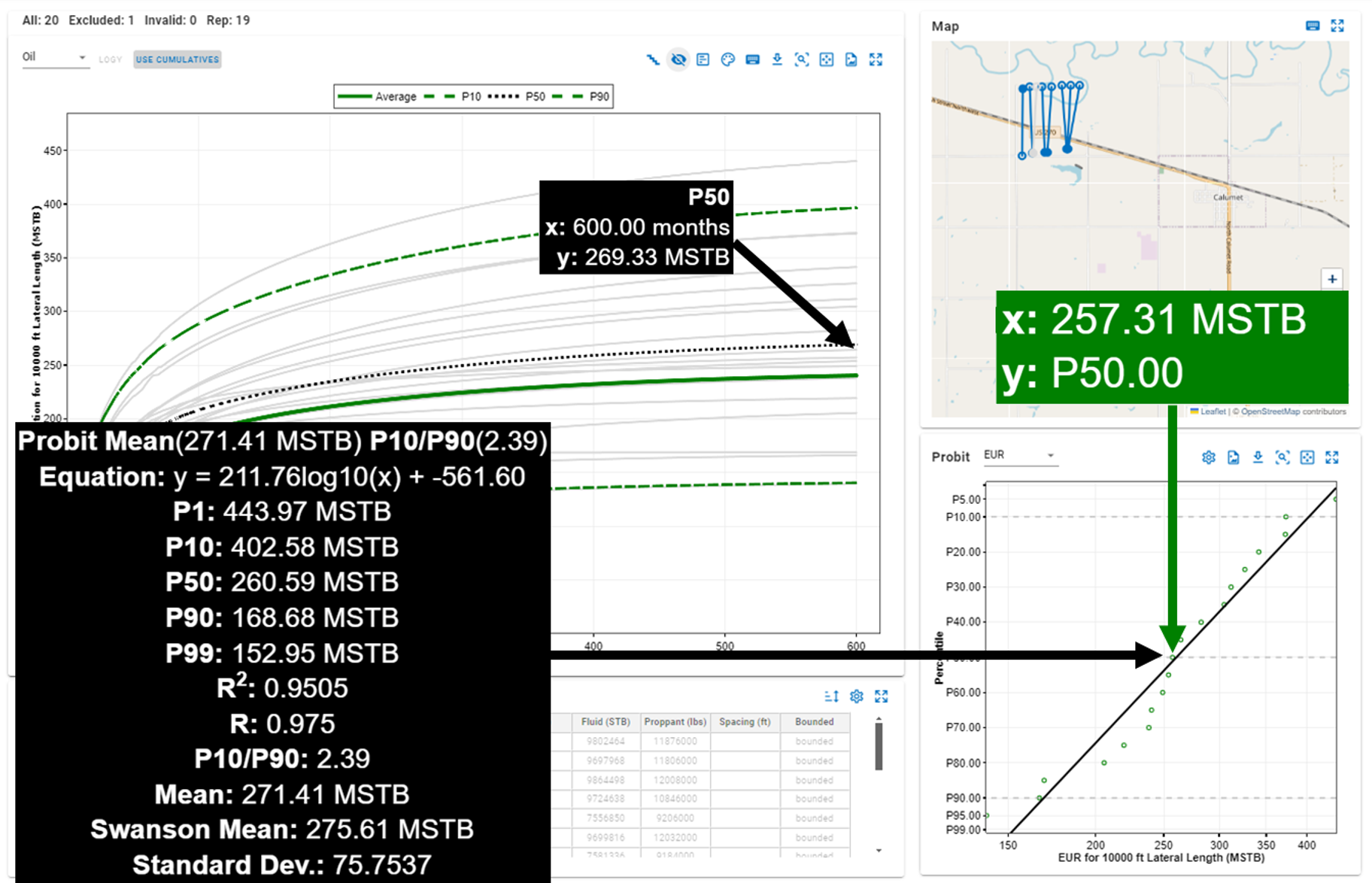
The probit plot calculates percentiles from the ranked values for the wells in the selected metric. It represents a single point in time or a single well-level metric, such as EUR.
7.2. Percentile Curves
Percentile curves calculate a given percentile (p) from the wells' values at each time step using linear interpolation.
7.3. Which approach is correct?
Both approaches are valid, but they answer different questions.
Probit Plot Percentiles: This approach ranks the available well-level values for one selected metric or point in time. It is useful for examining the distribution of a metric across the well population. The ranked values can also be used to assess the distribution and estimate uncertainty.
Linear Interpolation Percentiles: This approach calculates each percentile from its position within a sorted vector of values. It is used at every time step to construct a continuous percentile curve. Because the wells contributing to a percentile can change over time, a percentile curve does not generally represent one physical well.
Use the probit plot to analyze the distribution of a selected metric across wells. Use percentile curves to track a selected percentile over time.
7.4. Why isn't the cumulative P50 exactly the same as the EUR P50 in the probit plot?
The P50 value at each time step (and likewise the P10 or P90 value) is not linked to one actual well; it will usually reflect different wells over time. By contrast, the EUR P50 is calculated from the distribution of complete, well-level EUR values. Because a percentile operation and time integration are not interchangeable, the cumulative P50 curve and the P50 of the EUR distribution need not be identical, although they are often similar.
8. Type Well Diagnostic
-
The arithmetic mean is highly influenced by outliers and is not reliable as the sole basis for a Type Well diagnostic.
-
The geometric mean is less influenced by high-value outliers but is sensitive to very low values.
-
The P50 is robust to the magnitude of outliers because it depends primarily on the ordering of values.
-
Therefore, a new diagnostic is proposed for Type Well construction.
-
The deviation of the arithmetic and geometric means from P50 indicates data stability issues.
-
Stable periods of history should be relied on more than unstable periods of history.
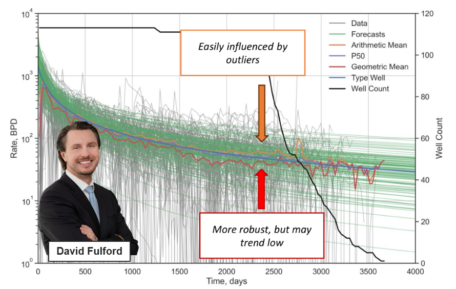
Courtesy: David Fulford
9. Related Properties
The Related Properties table provides the well-level properties associated with the Type Well population.
Available table actions include:
- Copy Table: copy the displayed Related Properties table to the clipboard.
- Export to Excel: export the Related Properties table to an Excel workbook.
These options are useful for QC, additional analysis, and sharing the Type Well input population.