Forecast Manager

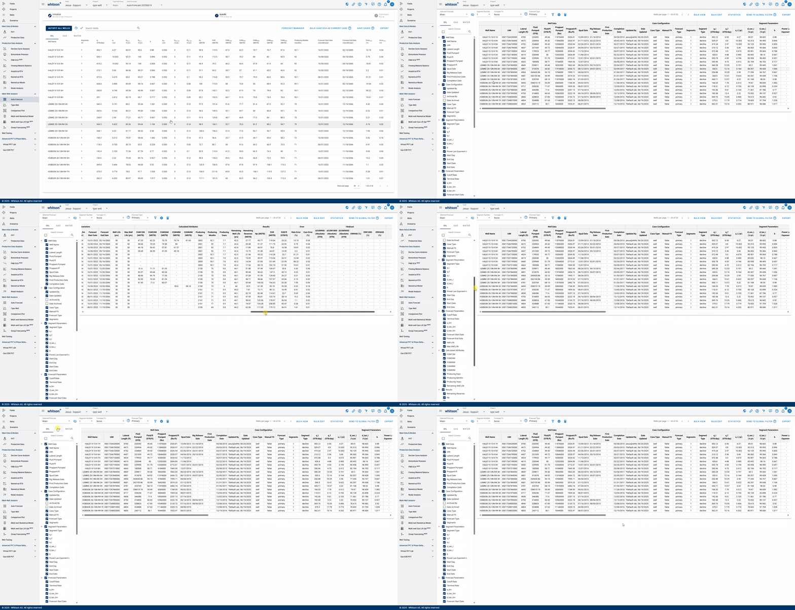
The Forecast Manager in whitson⁺ is a centralized workspace for reviewing, comparing, and validating production forecasts. Users can compare multiple forecast scenarios, such as reserves cases or prior AFEs, side-by-side using tools like unity plots, while also accessing detailed reporting of decline parameters. The GIF below shows how to access the Forecast Manager and begin exploring these workflows.

1. Overview

Selecting Forecast
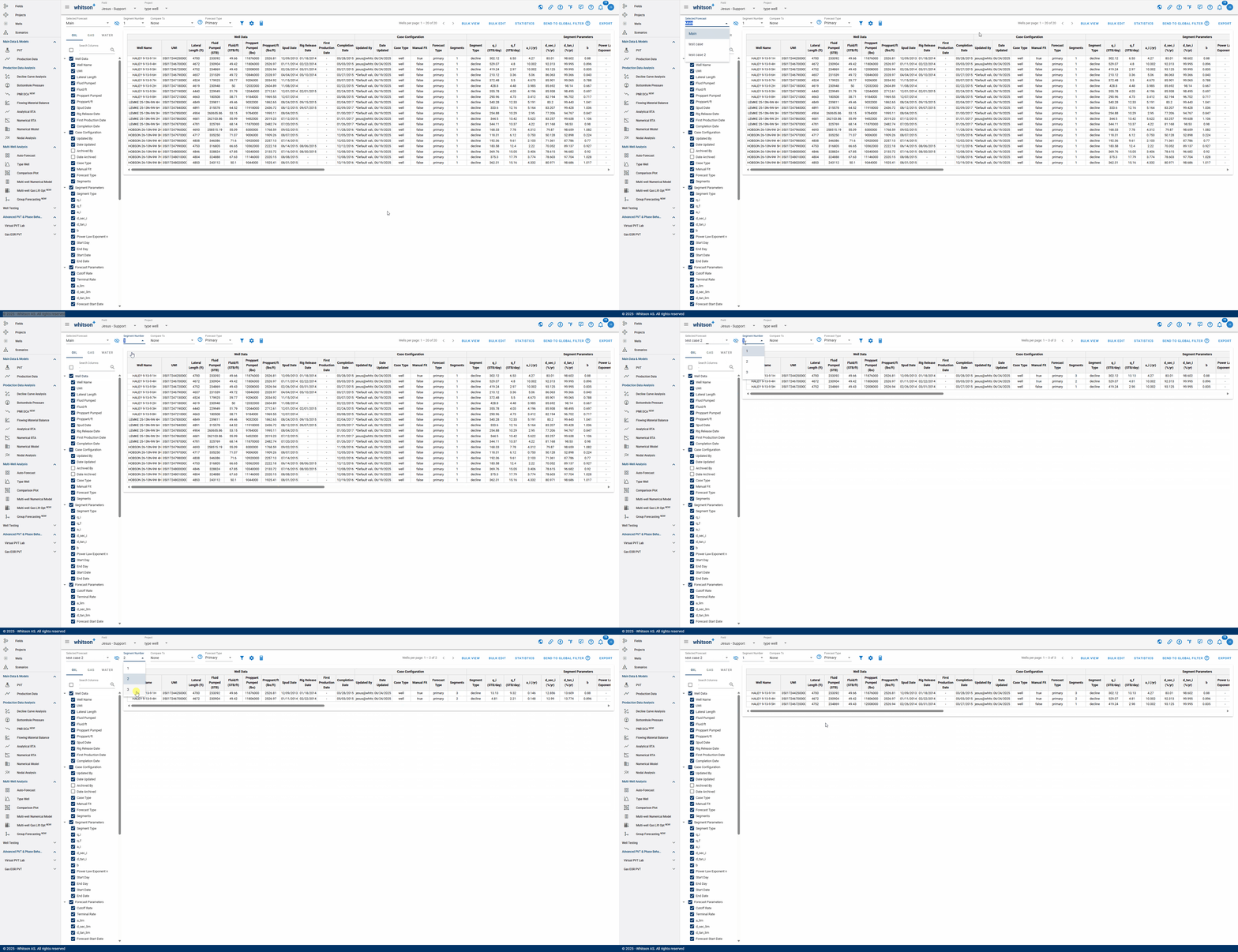
Choose a forecast case to display. Cases created in the Auto-Forecast section can be applied to all wells, while cases created in the Decline Curve Analysis section can be applied to individual wells.

Number of Segments
You can select the amount of segments included in the analysis. Additional segments can only be added manually to each well's analysis.

Comparing
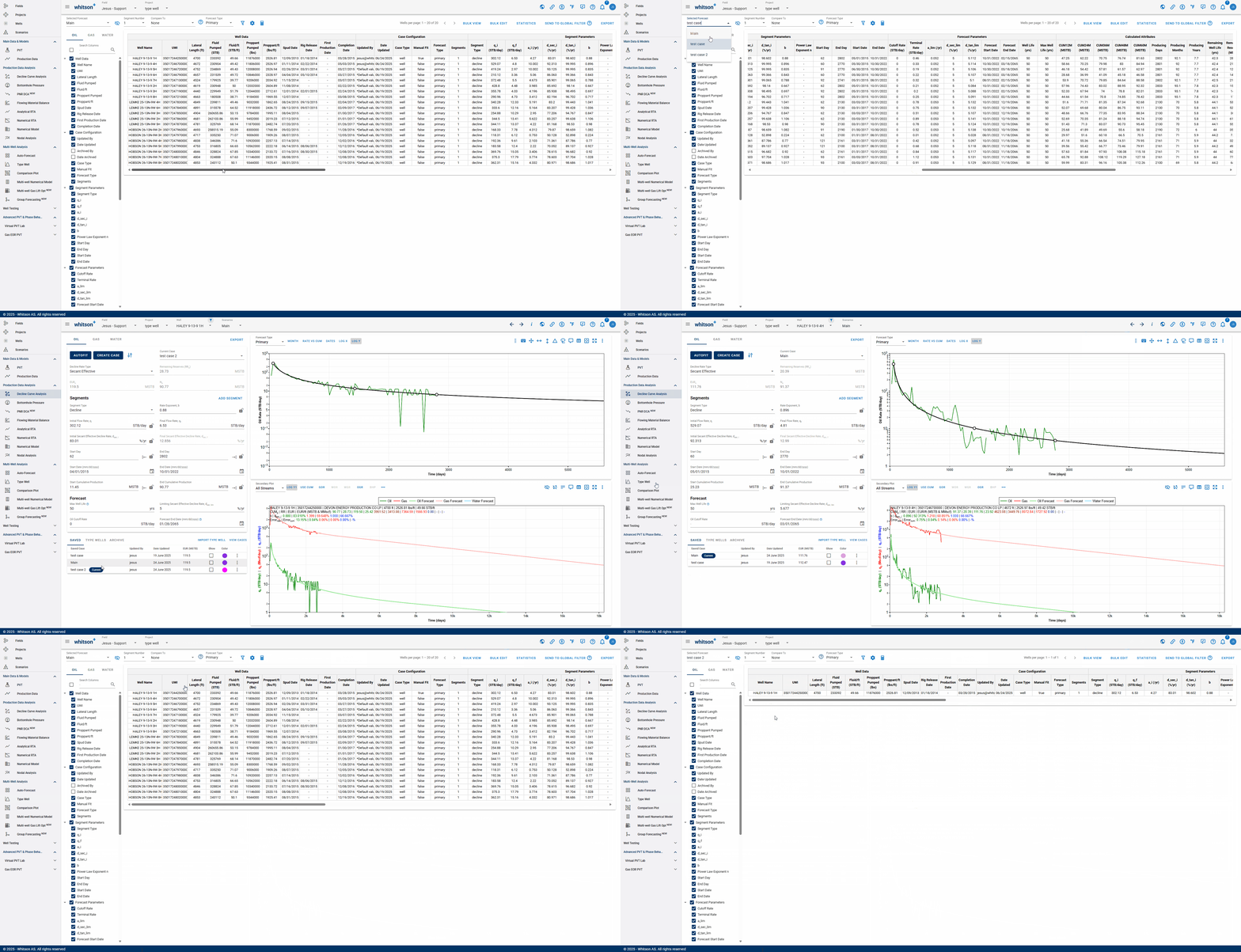
After selecting a comparison forecast, "Compare To" columns will populate at the end of the table, enabling variance analysis.

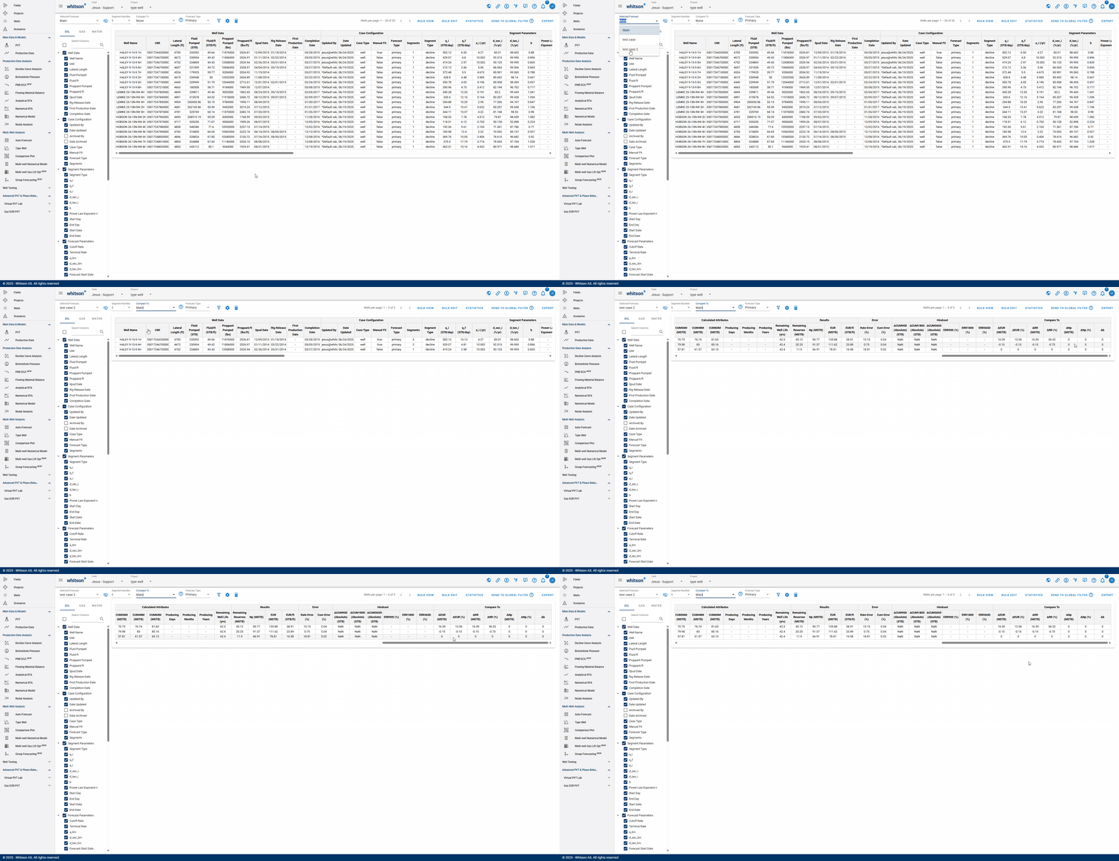
An interpretation of the gif above:

If the values are positive: "test case 2" is outperforming "Main"

If the values are negative: "Main" is outperforming "test case 2"

Forecast Type
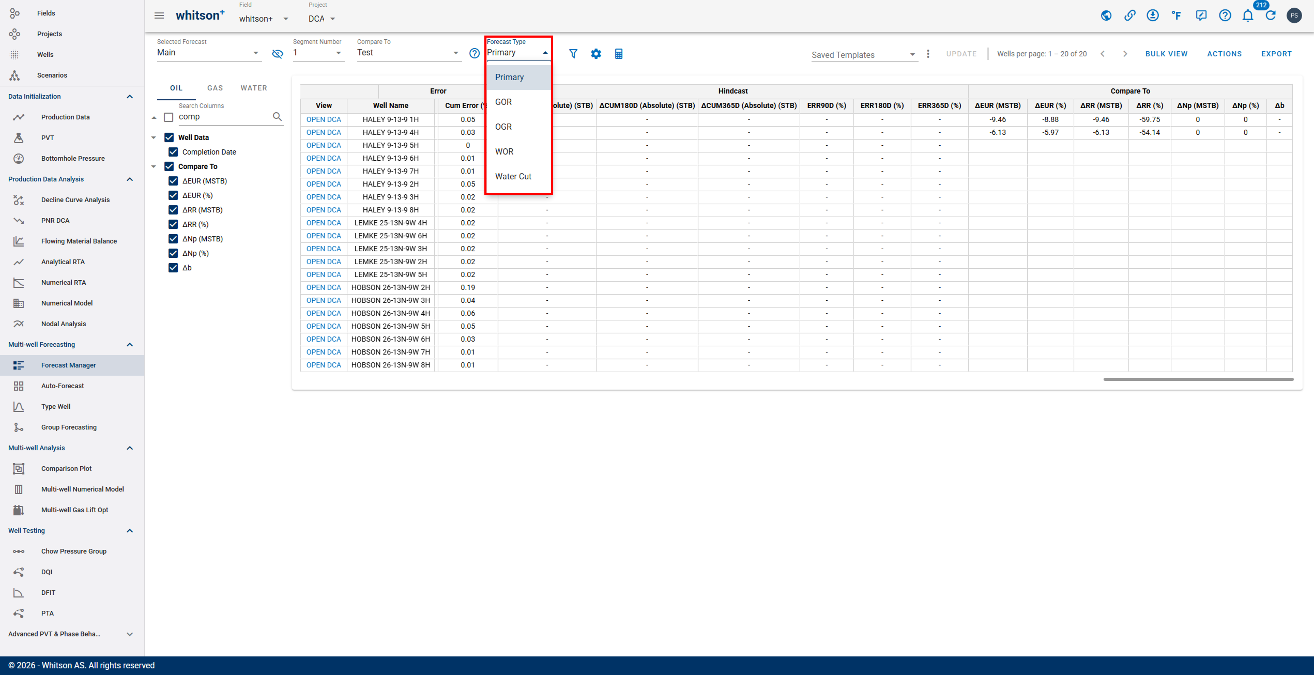
View the analysis by the type of forecast performed. The forecast type chosen must be tied to a previously saved case.

2. Filter

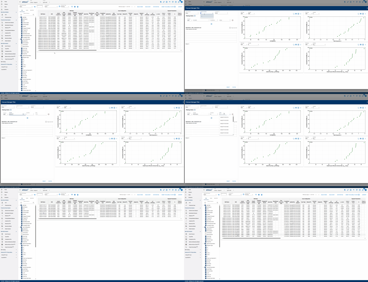
Allows you to filter wells based on different criteria:

• DCA Forecast: to filter by forecast saved case.

• Filter by Segments: to filter wells based on number of segments.

• Compare to: to filter by comparing two saved cases.

• Filtering Criteria: to filter wells based on a condition that a variable meets.

  • Variable: can be selected from a drop-down list, includes variables related to main well information & inputs, reservoir properties, completion metrics and well location information.
  • Condition: the following conditions can be selected from a drop-down list: equal to (=), less than (<), greater than (>), less than or equal to ($\leq$), greater than or equal to ($\geq$), not equal to ($\neq$) and case-sensitive text filtering on a string variable (in). For more specific filtering, you can add multiple conditions that will be combined using AND logic.
  • Value: the value associated with the condition.

• Well Name / UWI List: there are two filtering options. You can copy and paste a list of wells in a table format (the table will automatically expand to fit the data). Alternatively, you can copy and paste a list of wells as text, separated by commas.

Warning

RESET to remove all filters and see all the wells in the project.

2.1. Sorting

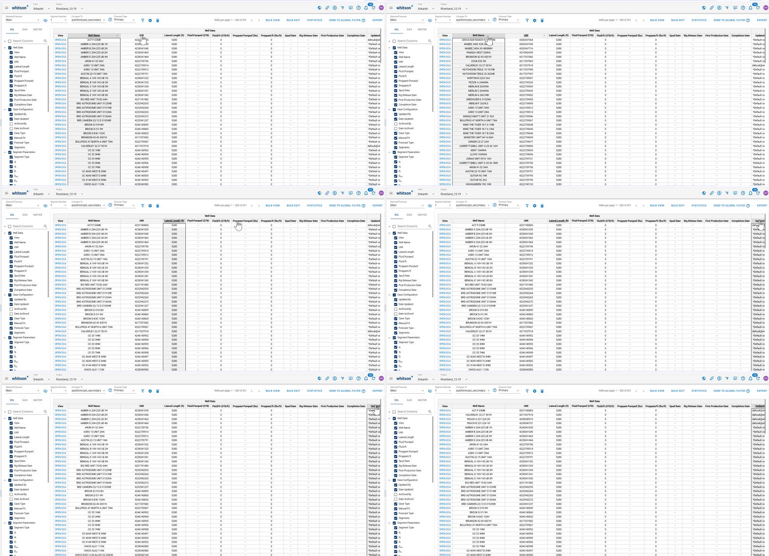
You can sort any table column by double-clicking the column header.

• Text columns (e.g., well name): sort alphabetically (A to Z or Z to A).
• Numeric columns (e.g., rates, depths): sort by value (low to high or high to low).

Double-click the header once to sort descending. Double-click the same header again to switch to ascending.

3. Hindcast

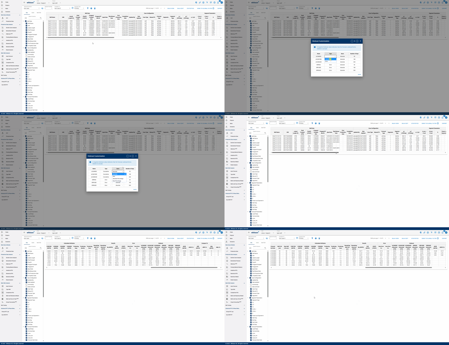
whitson⁺ offers hindcasting capabilities to evaluate the accuracy of auto-forecasted results. During the fitted period, users can report errors as absolute, real, or percentage values across a custom time range.

Default error metrics are provided but can be tailored within the Forecast Manager—even after new production data has been added post-forecast. Additionally, users can visually inspect forecast performance and back-calculate cumulative production directly in the platform.

Info

• A negative hindcast value indicates that the forecast underperforms relative to actuals.
• If any changes are made in the Hindcast Customization section, the hindcast must be calculated using the calculator icon.

3.1. Hindcast Metrics

The Hindcast analysis evaluates the Selected Forecast by comparing it with historical production over the selected hindcast period.

ERR_X_D

ERR_X_D is the Root Mean Square (RMS) of the percentage error between forecasted and historical production rates over the selected hindcast period. Historical data points with a production rate of zero are excluded from the calculation.

The percentage error at each valid time step is calculated as:

$$E_i = 100 \times \frac{q_{i,\mathrm{hist}} - q_{i,\mathrm{fcst}}}{q_{i,\mathrm{hist}}}$$

where:

• $q_{i,\mathrm{hist}}$ = historical production rate at time step $i$
• $q_{i,\mathrm{fcst}}$ = forecasted production rate at time step $i$

The ERR_X_D value is calculated as the Root Mean Square (RMS) of the percentage errors:

$$\mathrm{ERRXD} = \sqrt{\frac{1}{N}\sum_{i=1}^{N} E_i^2}$$

where:

• $N$ = number of valid time steps within the last 365 days
• Zero-rate historical points are excluded from the calculation.

CUM_X_D

CUM_X_D measures the difference between the forecasted and actual cumulative production over the last X days.

$$\mathrm{CUM365D} = (C_{\mathrm{fcst,end}} - C_{\mathrm{fcst,start}}) - (C_{\mathrm{hist,end}} - C_{\mathrm{hist,start}})$$

where:

• $C_{\mathrm{fcst,start}}$ = forecast cumulative production at the start of the 365-day window
• $C_{\mathrm{fcst,end}}$ = forecast cumulative production at the end of the 365-day window
• $C_{\mathrm{hist,start}}$ = historical cumulative production at the start of the 365-day window
• $C_{\mathrm{hist,end}}$ = historical cumulative production at the end of the 365-day window

A positive CUM_X_D indicates that the forecast predicts higher cumulative production than the actual production. A negative value indicates that the forecast underestimates cumulative production.

3.2. Hindcast Basis

The Basis option determines how the difference between the forecast and historical cumulative production is calculated over the selected hindcast period.

• Absolute – Sum of the absolute differences between forecast and historical cumulative values.
• Real – Sum of the signed differences between forecast and historical cumulative values.
• Absolute Percentage – Sum of the absolute percentage differences between forecast and historical cumulative values, relative to the historical values.
• Real Percentage – Sum of the signed percentage differences between forecast and historical cumulative values, relative to the historical values.

4. Bulk View

Allows you to view the DCA of up to eight wells simultaneously for comparison purposes.

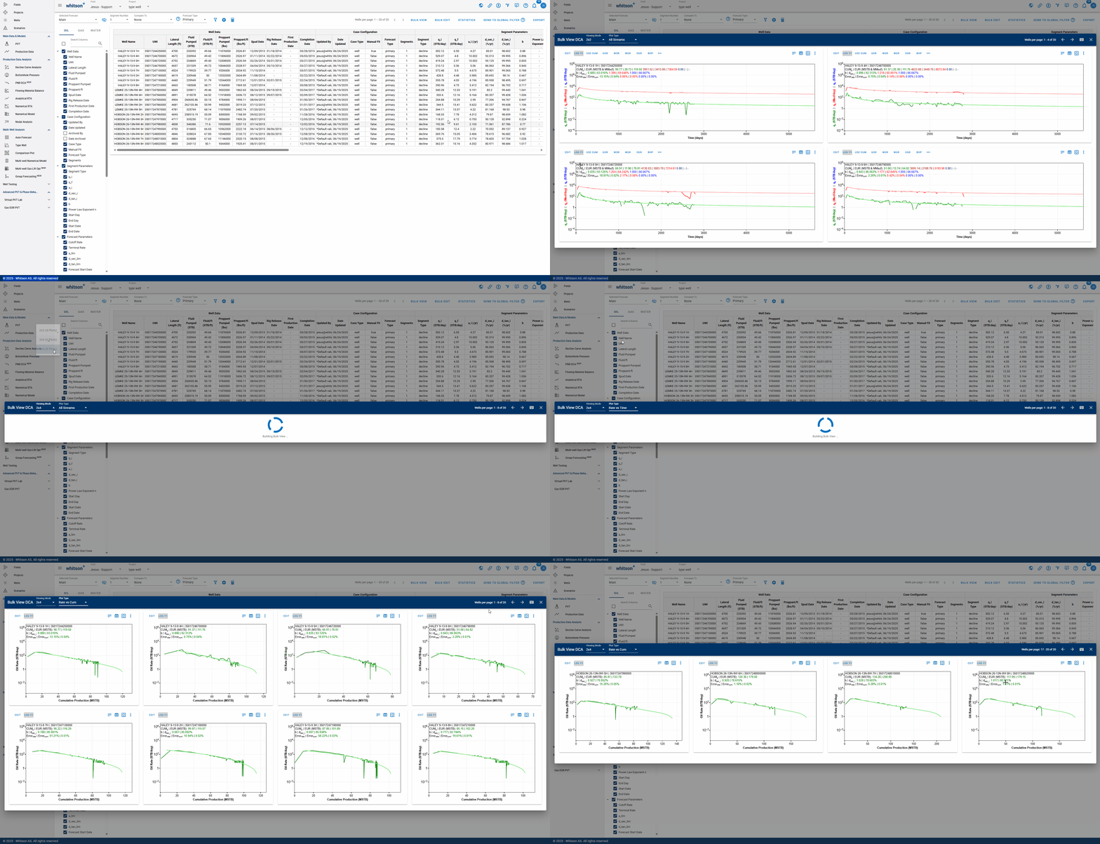
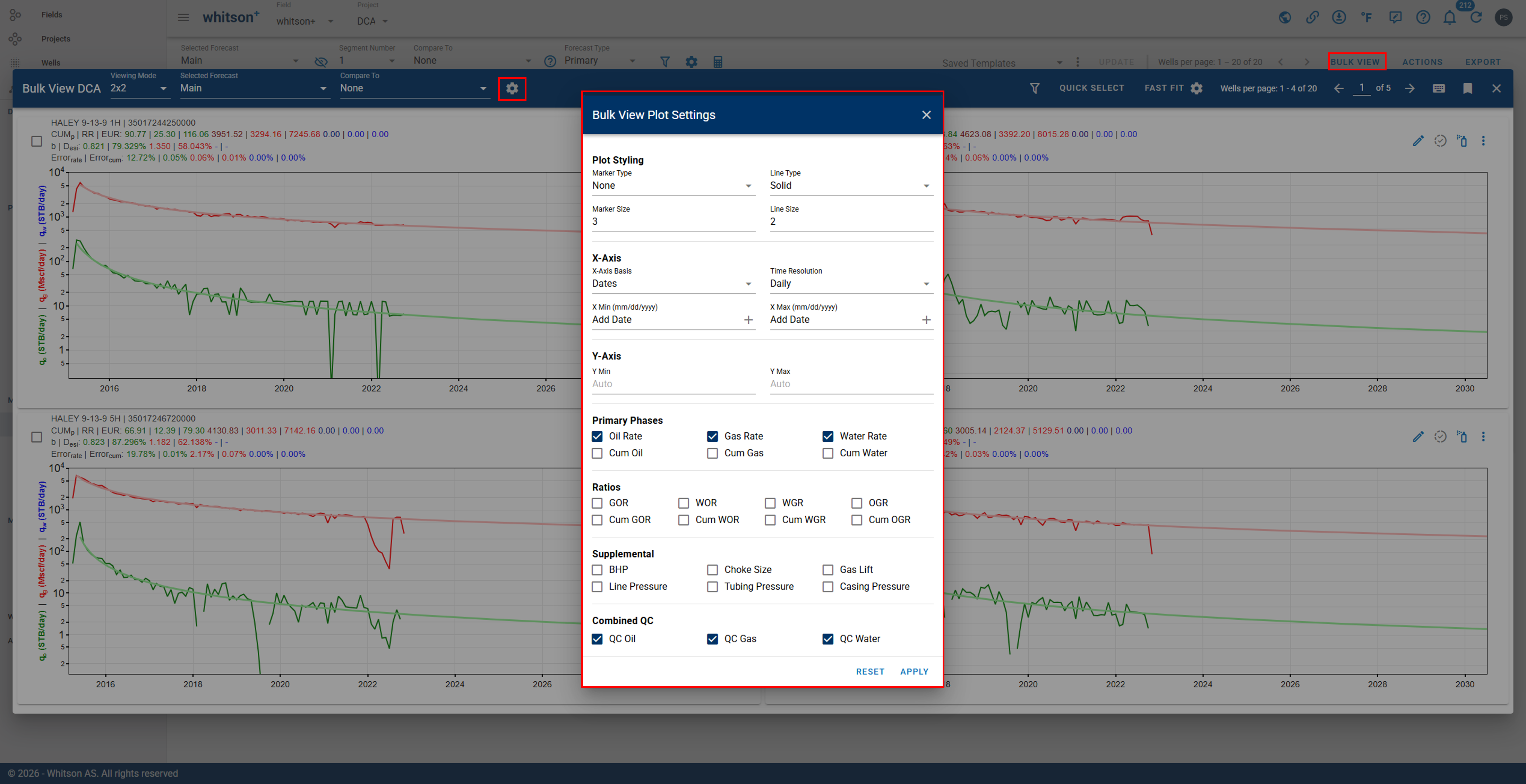
Bulk View let's you control what is displayed across the entire grid. Use the settings panel shown in the .gif above to:

• Choose the X-Axis Basis (e.g., Dates) and the Time Resolution (e.g., Daily).
• Toggle which curves appear on every plot:
  • Primary Phases: Oil, Gas, and Water rates, plus cumulative options.
  • Ratios: GOR, WOR, WGR, OGR, and cumulative ratio options.
  • Supplemental: BHP, Choke Size, Gas Lift, and surface pressures (Line, Tubing, Casing).

Click APPLY to update all eight plots at once, or RESET to return to default settings.

4.1. Fast Fit

The Fast Fit panel lets you bulk fit wells directly from Bulk View, without opening each well one-by-one. It is designed for quick QC and fast adjustments across the wells shown in the 2x4 grid.

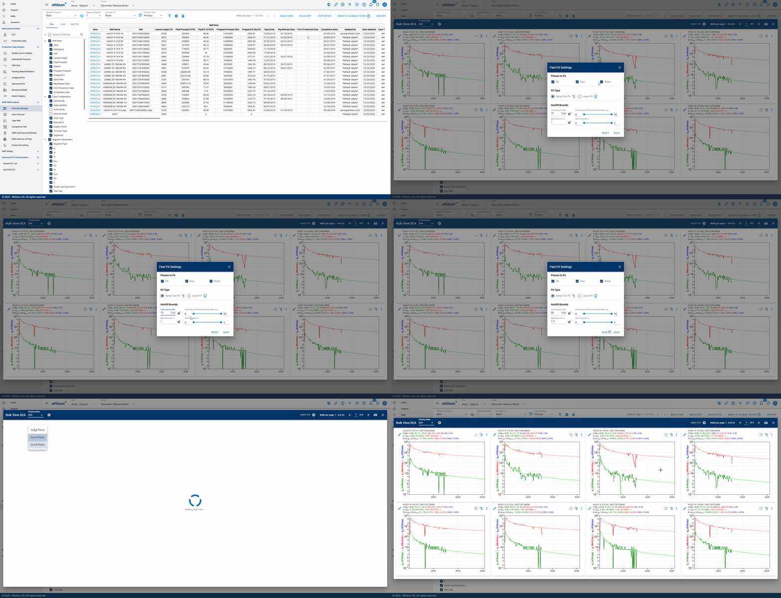
Use Fast Fit to:

• Select which phases to fit: Oil, Gas, and/or Water.
• Choose a Fit Type:
  • Spray Gun Fit: quickly applies a fit over the visible trend.
  • Lasso Fit: fits only the points you select.
• Set Autofit Bounds (with sliders) to control the allowed range for:
  • Initial secant effective decline rate, Dsei
  • Rate exponent, b
• Use the lock icons to hold values constant while you adjust the other bounds.

Click SAVE to apply the Fast Fit settings, or RESET to return to defaults.

4.2. Bulk View Plot Settings

Available Settings:

• Plot Styling – Configure the visual appearance of all plots, including plot style, line type, line width, and marker size.
• Axes – Configure the X- and Y-axis display by selecting the X-axis basis, time resolution, axis ranges, or enabling automatic Y-axis scaling.
• Primary Phases – Select the production data to display, including oil, gas, and water rates, as well as cumulative production.
• Ratios – Display production ratios such as GOR, WOR, WGR, OGR, and their cumulative equivalents.
• Supplemental Data – Overlay operational parameters, including BHP, line pressure, choke size, tubing pressure, gas lift, and casing pressure.
• Combined QC – Display QC Oil, QC Gas, and QC Water to compare quality-controlled production data with production trends.

5. Actions

5.1. Rollup

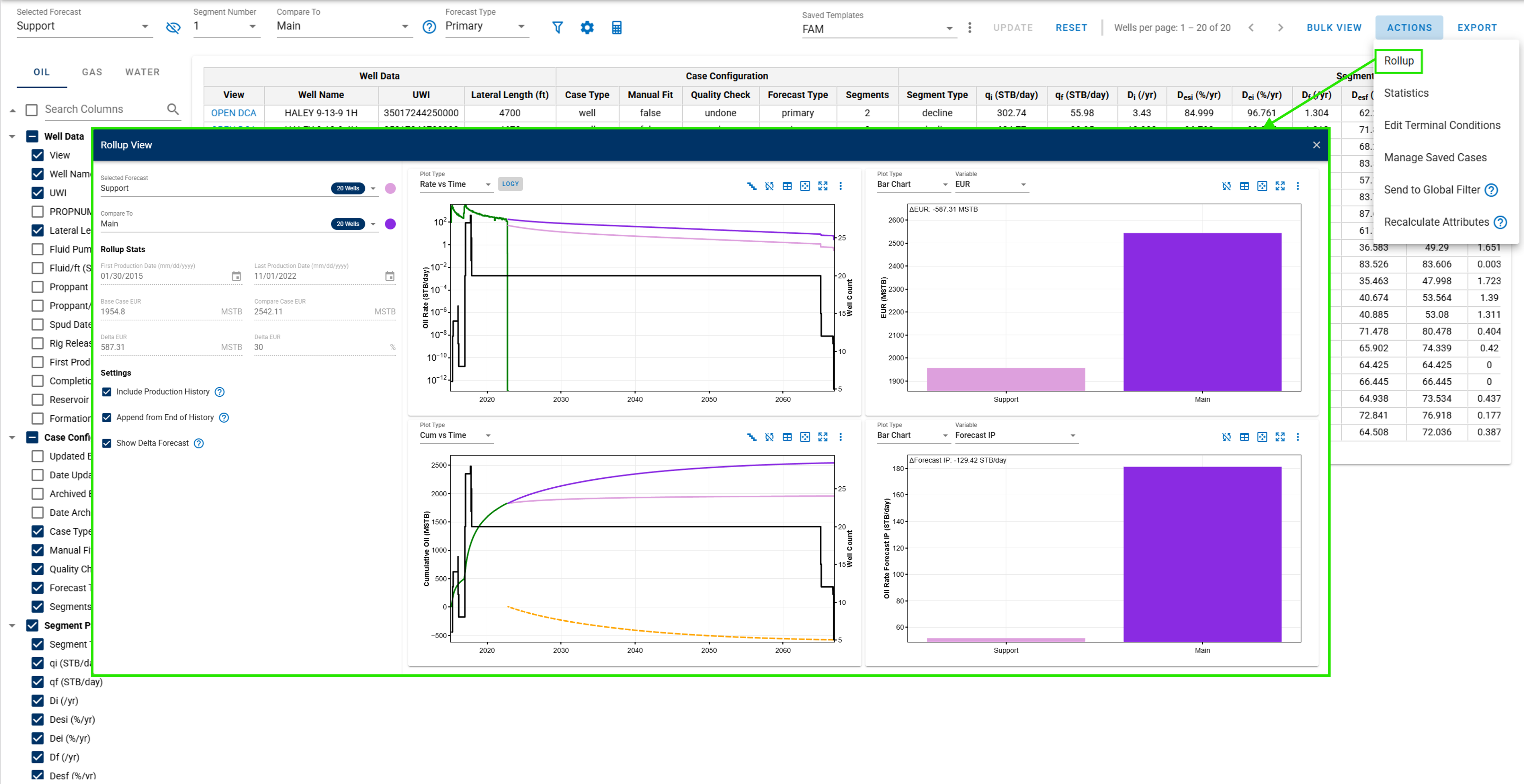
Rollup view that enables plotting two different aggregated forecasts in the same plot for convenience comparison.

• Enable Manage Saved Cases feature to the Actions button, making it easier to manage saved cases and perform bulk edits.

• Revamp Hindcast Customization settings, window, and calculation, including the option to use custom date ranges.

• Add PROPNUM as an available attribute selection for the table columns.

5.2. Statistics

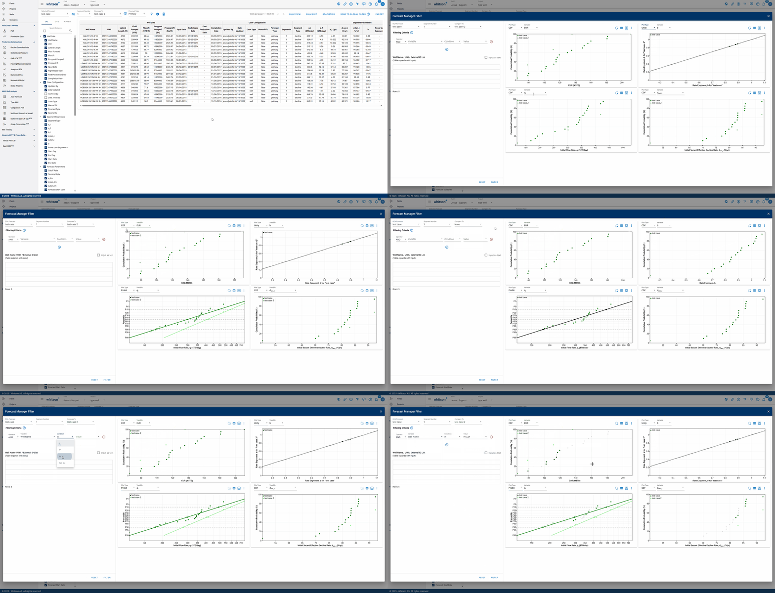
The Statistics feature provides visualization tools including; unity plots, cumulative distribution function (CDF) plots, and probit plots; for analyzing key decline parameters. Users can display up to four plots simultaneously and choose from a wide range of variables to visualize. These tools support filtering and quality control (QC), making it easy to validate and compare forecast results across wells, as demonstrated in the GIF below:

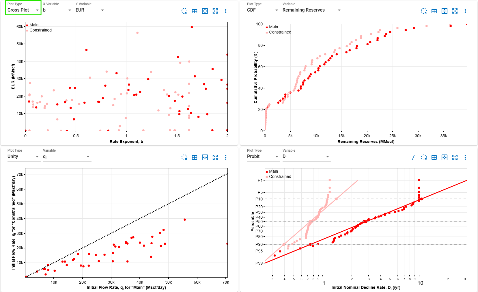
Cross plot in Forecast Manager: Add a new Plot Type in the Statistics section that enables users to create customizable cross plots.

5.3. Bulk Edit Terminal Conditions

Provides the ability to edit DCA settings for all wells at once.

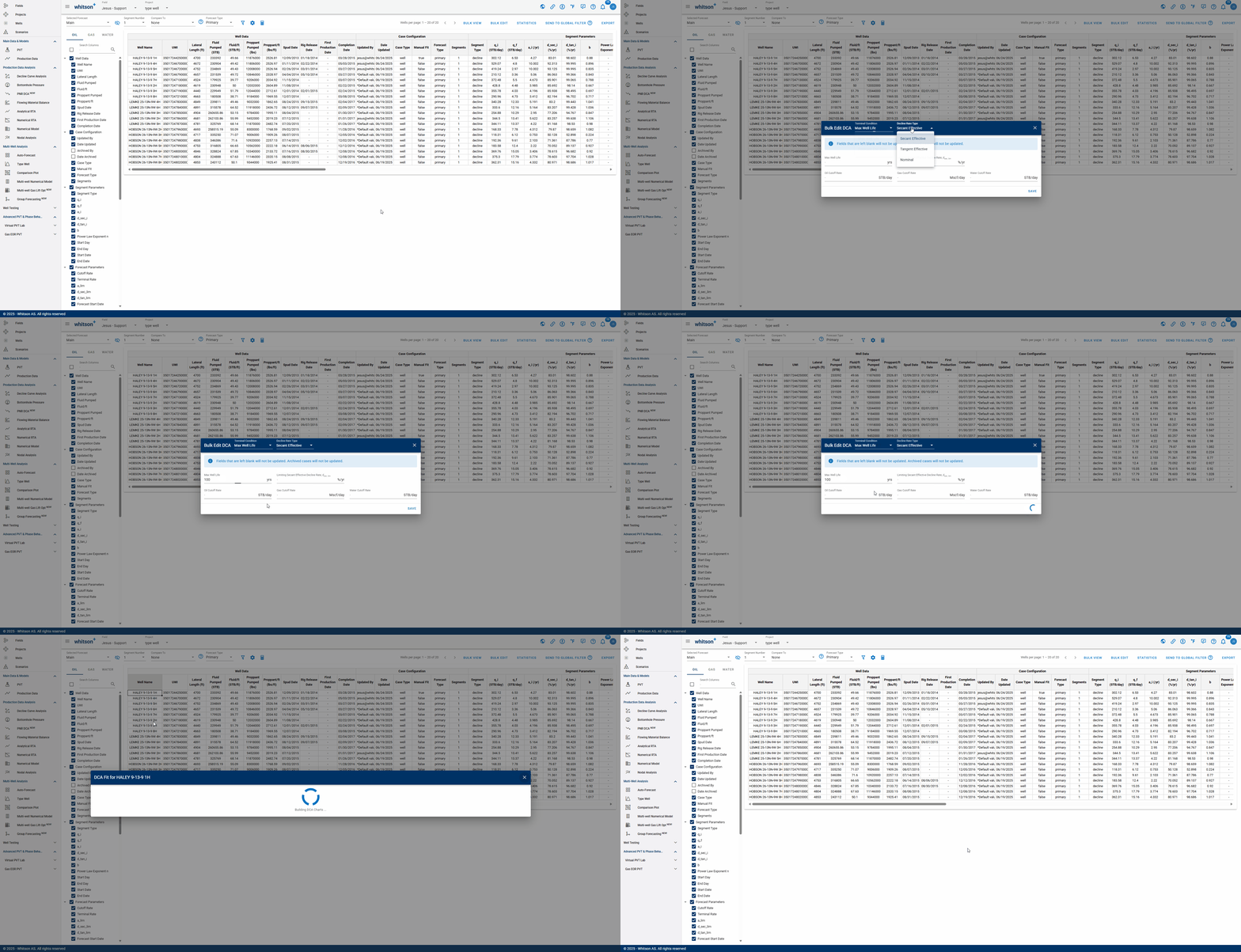
Info

Fields that are left blank will not be updated. Archived cases will not be updated.

The Edit Terminal Conditions module allows users to manually update the terminal conditions for one or more selected forecasts in the Forecast Manager.

Terminal Condition

Available options include:

• Max Well Life – Terminates the forecast after the specified production life.
• Forecast End Date – Terminates the forecast on a specified calendar date.

Selecting a terminal condition dynamically updates the corresponding input field.

Decline Rate Type

Specifies how the limiting decline rate is interpreted for the forecast termination.

Available options include:

• Tangent Effective
• Secant Effective
• Nominal

The selected decline rate type determines the label and interpretation of the limiting decline rate input.

Cutoff Rate

Specifies the minimum oil/gas/water production rates which the forecast is terminated.

5.4. Global Filter

Sends the selected forecast filter criteria to the global well filter. This applies the filter from the Forecast Manager across the entire platform. You can confirm this by navigating to the Wells page, where the filter will appear as active.

6. Export

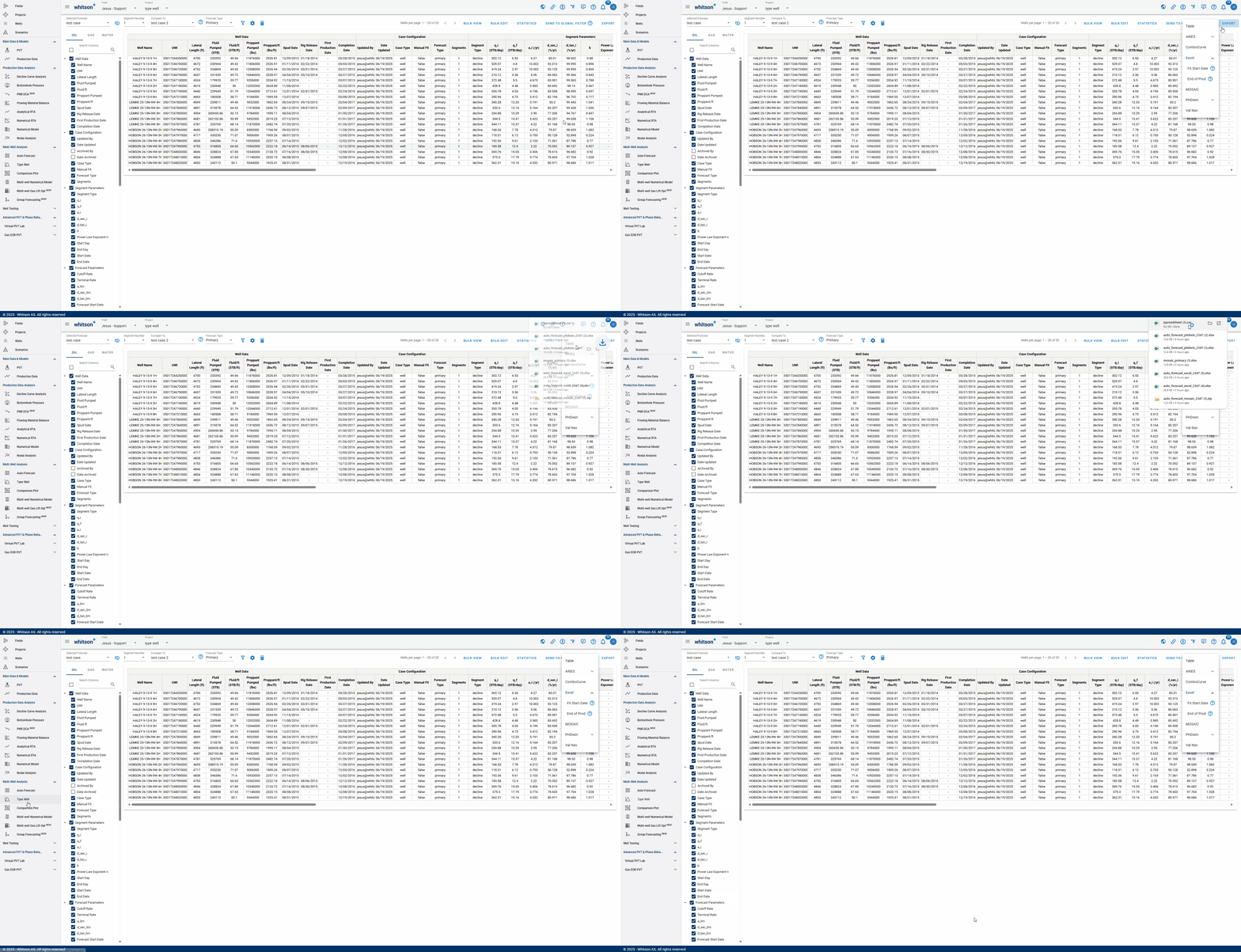
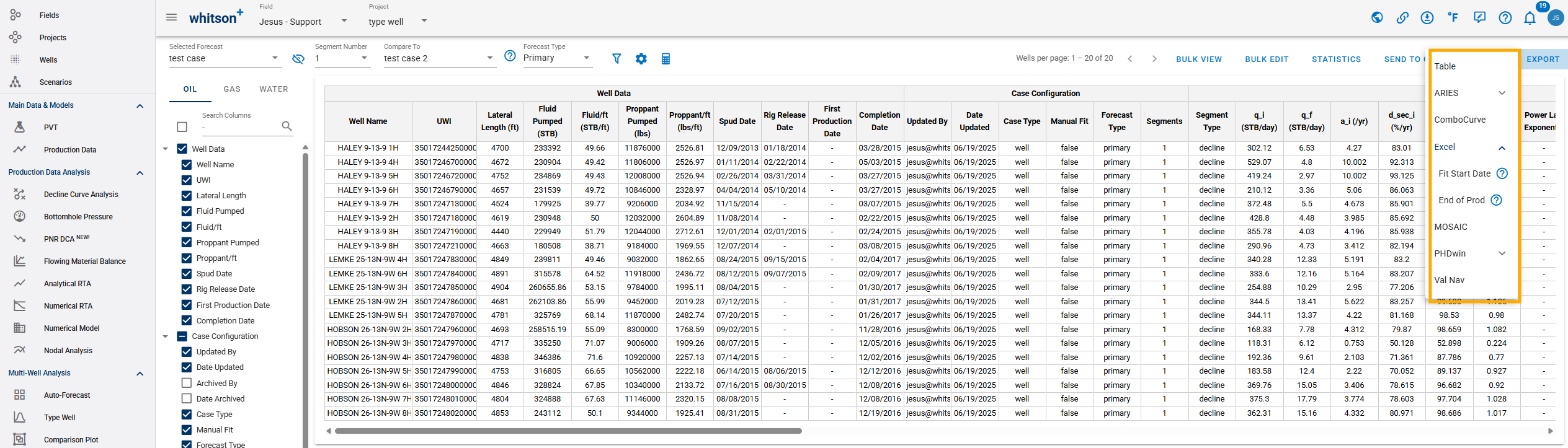
Click EXPORT up to the right to export to third-party software (for all streams). whitson⁺ supports the following for Forecast Manager:

• Table
• Aries
• Excel
• MOSAIC
• PHDwin
• Power Point
• Val Nav

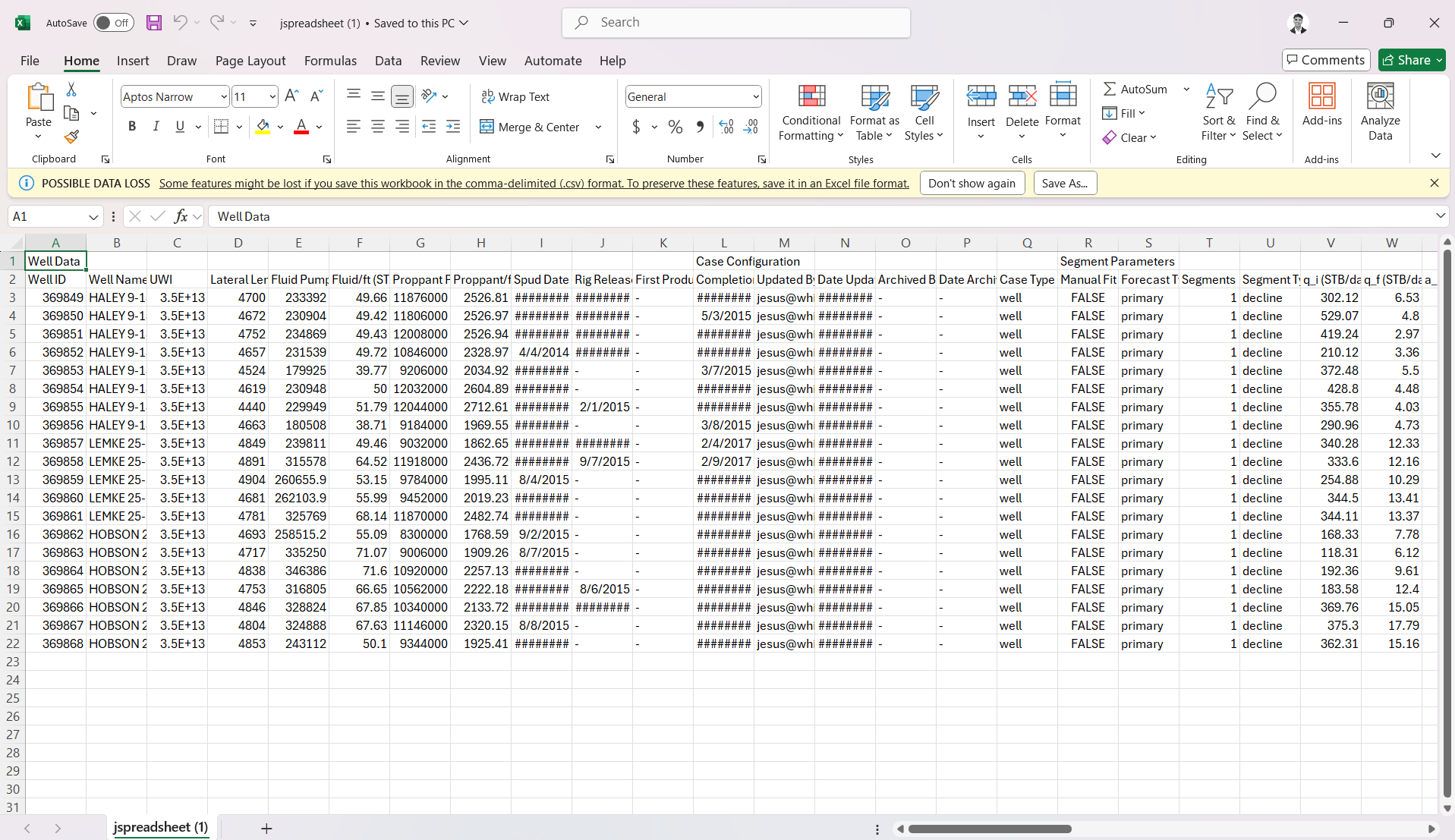
Forecast Manager Table

You can use this option to bulk export all well declines in the form of a table.

Here's an example of what that looks like - jspreadsheet.csv