Static Material Balance

1. Overview

1.1. Purpose and scope

Static material balance (MB) estimates the original hydrocarbons in place and identifies the energy sources driving a reservoir, using cumulative production and injection, fluid (PVT) properties, and static (shut-in, stabilized) average reservoir pressures. It is called “static” to distinguish it from flowing material balance, which uses flowing pressures and rates instead of shut-in pressure surveys.

This module covers:

• the general material balance equation (MBE) and the meaning of each term;
• dry-gas material balance, including the corrected ($p/Z^{**}$) formulation for overpressured, water-drive and connected reservoirs;
• oil material balance using linearized (Havlena–Odeh) plots, pressure matching, drive indices and diagnostic plots;
• the generalized formulation for volatile oils.

1.2. The tank model

Material balance treats the reservoir as a single tank. The underlying assumptions are:

1. Zero-dimensional reservoir. At any time, one average pressure (referred to a common datum) describes the whole connected pore volume, and fluid properties are uniform.
2. Isothermal depletion. Reservoir temperature is constant.
3. Phase equilibrium. Oil and gas in the reservoir are in equilibrium at the average pressure; PVT properties from laboratory tests represent reservoir behaviour.
4. Cumulative, not incremental, balance. The equation always compares the current state at pressure $p$ with the initial state at $p_{i}$. It is not evaluated step by step, except for time-dependent influx terms.
5. Time-independence of the tank terms. Only aquifer and connected-tank influx depend explicitly on time; all other terms depend on pressure alone.

Because there is no geometry and no flow equation, the tank model cannot predict how fluids move within the reservoir — only how much expansion must have occurred to explain the observed withdrawal.

1.3. Data requirements

The reliability of a material balance analysis is governed almost entirely by the input data:

Data	Requirement
Production and injection	Cumulative oil, gas and water produced, and gas and water injected, for every well completed in the reservoir. Missing wells or misallocated volumes bias the result.
Static pressure	An initial pressure and several stabilized shut-in pressures over the producing life, corrected to a common datum. Pressures from low-permeability wells that were not shut in long enough will read low.
PVT	Validated \(B_{o}\), \(R_{s}\), \(B_{g}\) (or \(Z\)), \(B_{w}\) and, for volatile systems, \(R_{v}\), ideally from representative bottomhole or recombined samples.
Rock and water	Pore-volume compressibility \(c_{f}\), water compressibility \(c_{w}\) and initial water saturation \(S_{wi}\).
Geology (optional)	Volumetric estimates of \(N\), \(G\) or gas-cap size \(m\) to constrain non-unique solutions.

1.4. Average reservoir pressure

Every pressure-dependent quantity in the MBE must be evaluated at the volume-averaged reservoir pressure. Individual well pressures are first referred to a common datum,

$$\begin{equation} \label{SMB-1} p_{\text{datum}} = p_{\text{gauge}} + \frac{\rho g}{144\, g_{c}}\left( D_{\text{datum}} - D_{\text{gauge}} \right)\tag{1} \end{equation}$$

where $\rho$ is the density of the continuous fluid between the gauge and the datum (lbm/ft³), and depths are true vertical depths (ft). The reservoir average is then weighted by the pore volume drained by each well:

$$\begin{equation} \label{SMB-2} \bar{p} = \frac{\sum_{j}^{}p_{j}V_{j}}{\sum_{j}^{}V_{j}},\quad\quad V_{j} \propto \frac{q_{j}}{\left| \, dp_{j}/dt\, \right|}\tag{2} \end{equation}$$

The second relation follows from the definition of compressibility applied to each drainage volume under pseudo-steady state: a well that withdraws at rate $q_{j}$ while its pressure falls at $dp_{j}/dt$ drains a pore volume proportional to their ratio. When drainage volumes are unknown, a simple arithmetic average of datum-corrected pressures is a common fallback.

2. The General Material Balance Equation

2.1. Volume balance concept

Consider the reservoir at initial pressure $p_{i}$ and again after the average pressure has dropped to $p$ (Figure 1). If the fluids that remained in the reservoir were allowed to expand freely, they would occupy a volume larger than the original pore space. That excess must equal the volume — at reservoir conditions and pressure $p$ — of everything that left the reservoir, less what entered it:

$$\text{Net underground withdrawal} = \text{Expansion of reservoir fluids and rock} + \text{Net influx}$$

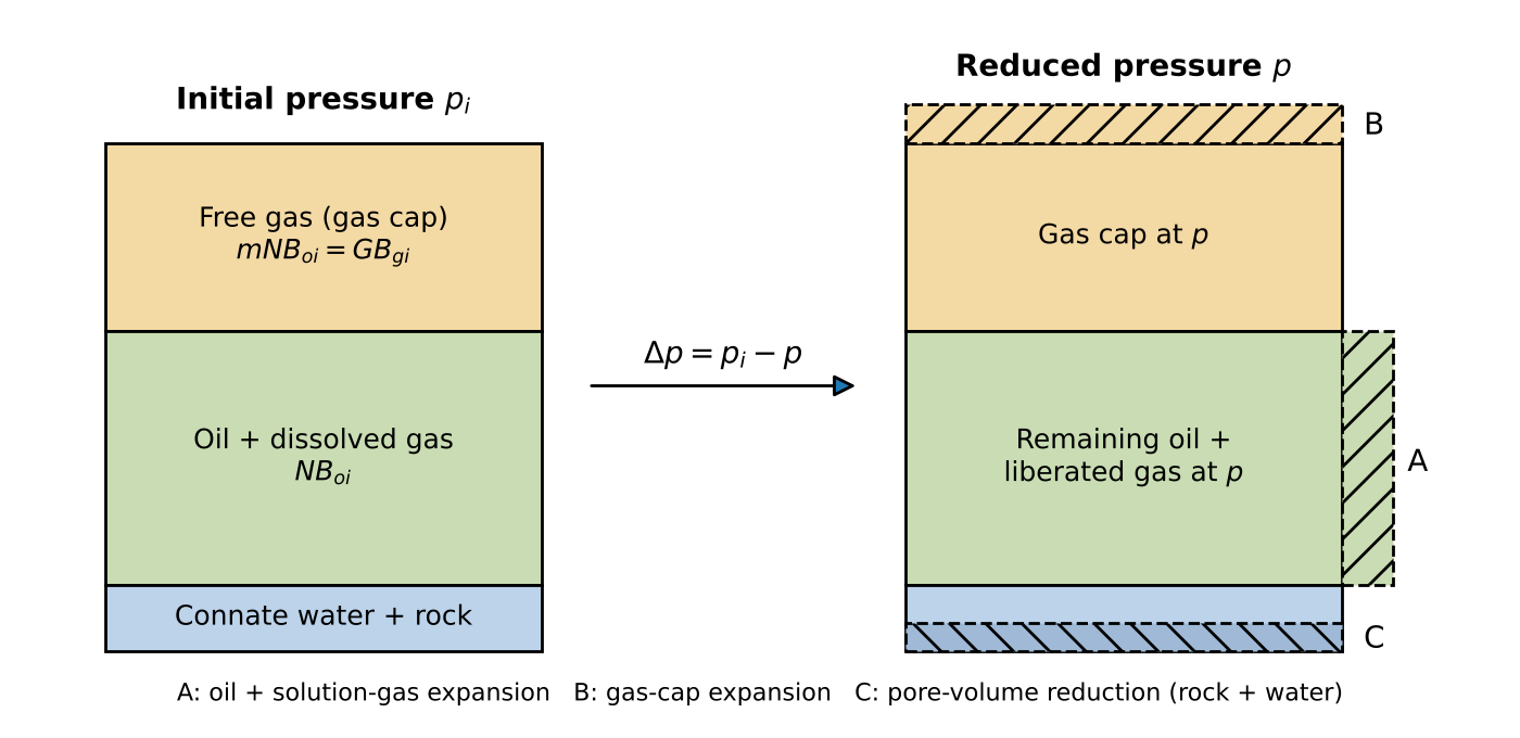Figure 1. Volume changes in the tank when pressure drops from $p_{i}$ to $p$. Expansion volumes A, B and C must accommodate the withdrawn fluids.

2.2. Definitions

Symbol	Definition	Units
\(N\)	Original oil in place	STB
\(G\)	Original free gas in place (gas cap, or the whole reservoir for a gas reservoir)	scf
\(m\)	Ratio of initial gas-cap volume to initial oil-zone volume, \(m = GB_{gi}/\left(NB_{oi}\right)\)	–
\(N_{p}\), \(G_{p}\), \(W_{p}\)	Cumulative oil, gas and water produced	STB, scf, STB
\(R_{p}\)	Cumulative produced gas–oil ratio, \(G_{p}/N_{p}\)	scf/STB
\(W_{inj}\), \(G_{inj}\)	Cumulative water and gas injected	STB, scf
\(W_{e}\)	Cumulative water influx from the aquifer	STB
\(\Delta p\)	Pressure drop, \(p_{i} - p\)	psi

2.3. Derivation

Each expansion term is the difference between the reservoir volume a fixed quantity of material occupies at $p$ and at $p_{i}$.

(a) Oil and its originally dissolved gas. $N$ stock-tank barrels occupy $NB_{oi}$ at $p_{i}$ and $NB_{o}$ at $p$. Below the bubble point, the gas released from solution, $N\left( R_{si} - R_{s} \right)$ scf, occupies $N\left( R_{si} - R_{s} \right)B_{g}$ at $p$. The total expansion is

$$\begin{equation} \label{SMB-3} \Delta V_{o} = N\left\lbrack \left( B_{o} - B_{oi} \right) + \left( R_{si} - R_{s} \right)B_{g} \right\rbrack\tag{3} \end{equation}$$

(b) Gas-cap gas. The free gas $G = mNB_{oi}/B_{gi}$ occupies $GB_{gi}$ at $p_{i}$ and $GB_{g}$ at $p$:

$$\begin{equation} \label{SMB-4} \Delta V_{g} = G\left( B_{g} - B_{gi} \right) = mNB_{oi}\left( \frac{B_{g}}{B_{gi}} - 1 \right)\tag{4} \end{equation}$$

(c) Connate water expansion and pore-volume reduction. As pressure falls, connate water expands and the pore space contracts; both reduce the space available to hydrocarbons. With the definitions

$$\begin{equation} \label{SMB-5} c_{w} = - \frac{1}{V_{w}}\frac{dV_{w}}{dp},\quad\quad c_{f} = \frac{1}{V_{p}}\frac{dV_{p}}{dp}\tag{5} \end{equation}$$

integration from $p_{i}$ to $p$ gives the water and pore volumes at $p$:

$$\begin{equation} \label{SMB-6} V_{w} = V_{wi}\exp\left( \int_{p}^{p_{i}}c_{w}\, dp' \right),\quad\quad V_{p} = V_{pi}\exp\left( - \int_{p}^{p_{i}}c_{f}\, dp' \right)\tag{6} \end{equation}$$

The reduction in hydrocarbon pore volume (HCPV $= V_{p} - V_{w}$) relative to its initial value $V_{pi}\left( 1 - S_{wi} \right)$ is therefore

$$\begin{equation} \label{SMB-7} \varepsilon_{fw} \equiv \frac{\Delta\left( \text{HCPV} \right)}{\text{HCPV}_{i}} = \frac{S_{wi}\left\lbrack \exp\left( \int_{p}^{p_{i}}c_{w}\, dp' \right) - 1 \right\rbrack + \left\lbrack 1 - \exp\left( - \int_{p}^{p_{i}}c_{f}\, dp' \right) \right\rbrack}{1 - S_{wi}}\tag{7} \end{equation}$$

This is the rigorous form. For constant, small compressibilities, $e^{x} \approx 1 + x$ and $\varepsilon_{fw}$ reduces to the familiar approximation

$$\begin{equation} \label{SMB-8} \varepsilon_{fw} \approx \frac{c_{w}S_{wi} + c_{f}}{1 - S_{wi}}\,\Delta p\tag{8} \end{equation}$$

Since the initial HCPV is $(1 + m)NB_{oi}$, the volume contributed by this mechanism is

$$\begin{equation} \label{SMB-9} \Delta V_{fw} = (1 + m)\, NB_{oi}\,\varepsilon_{fw}\tag{9} \end{equation}$$

(d) Underground withdrawal. The produced oil, $N_{p}$, occupies $N_{p}B_{o}$ at $p$ and carries $N_{p}R_{s}$ scf of gas in solution. The remaining produced gas, $N_{p}\left( R_{p} - R_{s} \right)$, was free gas in the reservoir and occupies $N_{p}\left( R_{p} - R_{s} \right)B_{g}$. Adding produced water and subtracting injected fluids:

$$\begin{equation} \label{SMB-10} F = N_{p}\left\lbrack B_{o} + \left( R_{p} - R_{s} \right)B_{g} \right\rbrack + W_{p}B_{w} - W_{inj}B_{w} - G_{inj}B_{g,inj}\tag{10} \end{equation}$$

(e) Water influx. Aquifer water entering the tank displaces an equal reservoir volume, $W_{e}B_{w}$.

Equating withdrawal to the sum of (a), (b), (c) and (e):

$$\begin{equation} \label{SMB-11} N_{p}\left\lbrack B_{o} + \left( R_{p} - R_{s} \right)B_{g} \right\rbrack + \left( W_{p} - W_{inj} \right)B_{w} - G_{inj}B_{g,inj} = N\left\lbrack \left( B_{o} - B_{oi} \right) + \left( R_{si} - R_{s} \right)B_{g} \right\rbrack + mNB_{oi}\left( \frac{B_{g}}{B_{gi}} - 1 \right) + (1 + m)NB_{oi}\,\varepsilon_{fw} + W_{e}B_{w}\tag{11} \end{equation}$$

2.4. Compact form

Following Havlena and Odeh, define the expansion terms per stock-tank barrel of oil:

$$\begin{equation} \label{SMB-12} E_{o} = \left( B_{o} - B_{oi} \right) + \left( R_{si} - R_{s} \right)B_{g}\tag{12} \end{equation}$$

$$\begin{equation} \label{SMB-13} E_{g} = B_{oi}\left( \frac{B_{g}}{B_{gi}} - 1 \right)\tag{13} \end{equation}$$

$$\begin{equation} \label{SMB-14} E_{fw} = (1 + m)\, B_{oi}\,\varepsilon_{fw}\tag{14} \end{equation}$$

Equation (11) then becomes

$$\begin{equation} \label{SMB-15} F = N\left( E_{o} + mE_{g} + E_{fw} \right) + W_{e}B_{w} = NE_{t} + W_{e}B_{w}\tag{15} \end{equation}$$

where $E_{t}$ is the total expansion per STB. An equivalent form, written in terms of the free gas in place $G$ rather than $m$ (using $mNB_{oi} = GB_{gi}$), separates the oil-zone and gas-cap contributions:

$$\begin{equation} \label{SMB-16} F - W_{e}B_{w} = N\left( E_{o} + B_{oi}\,\varepsilon_{fw} \right) + G\left( B_{g} - B_{gi} + B_{gi}\,\varepsilon_{fw} \right)\tag{16} \end{equation}$$

Equation (16) is the starting point for most of the oil analyses in Section 4.

2.5. Summary of terms

Term	Physical Meaning
\(F\)	Net reservoir volume removed: production at reservoir conditions minus injection.
\(NE_{o}\)	Swelling of the remaining oil plus the volume of gas liberated from it. Above the bubble point only liquid expansion contributes.
\(NmE_{g}\)	Expansion of the initial gas cap into space once occupied by oil.
\(NE_{fw}\)	Space released by connate-water expansion and pore compaction. Small in normally pressured reservoirs, significant in undersaturated or overpressured ones.
\(W_{e}B_{w}\)	Water encroaching from a connected aquifer.

Terms that do not apply to a given reservoir drop out: with no gas cap, $m = 0$ (and $G = 0$); with no aquifer, $W_{e} = 0$.

2.6. Undersaturated oil

Above the bubble point $R_{s} = R_{si} = R_{p}$ and no free gas exists. Writing the oil expansion through its isothermal compressibility, $B_{o} - B_{oi} = B_{oi}{\bar{c}}_{o}\,\Delta p$, Eq. (15) becomes

$$\begin{equation} \label{SMB-17} N_{p}B_{o} + \left( W_{p} - W_{inj} \right)B_{w} = NB_{oi}\left( \frac{{\bar{c}}_{o}S_{oi} + c_{w}S_{wi} + c_{f}}{1 - S_{wi}} \right)\Delta p + W_{e}B_{w} = NB_{oi}\, c_{e}\,\Delta p + W_{e}B_{w}\tag{17} \end{equation}$$

where $S_{oi} = 1 - S_{wi}$ and $c_{e}$ is the effective compressibility of the oil zone. Rock and water compressibility are of the same order as oil compressibility here, so $E_{fw}$ must not be neglected.

3. Gas Material Balance

3.1. Volumetric dry gas

For a dry-gas reservoir with no aquifer and negligible rock and water expansion, all terms except gas expansion vanish. Equation (16) with $N = 0$ reduces to

$$\begin{equation} \label{SMB-18} G_{p}B_{g} = G\left( B_{g} - B_{gi} \right)\quad \Rightarrow \quad GB_{gi} = \left( G - G_{p} \right)B_{g}\tag{18} \end{equation}$$

i.e. the gas remaining in the reservoir occupies the original gas pore volume. The gas formation volume factor follows from the real-gas law applied at reservoir and standard conditions ($Z_{sc} = 1$):

$$\begin{equation} \label{SMB-19} B_{g} = \frac{p_{sc}}{T_{sc}}\frac{ZT}{p} = 0.02827\,\frac{ZT}{p}\ \ \text{ft}^{3}/\text{scf} = 0.005035\,\frac{ZT}{p}\ \ \text{rb/scf}\tag{19} \end{equation}$$

with $T$ in °R and $p$ in psia. Substituting Eq. (19) into Eq. (18) and cancelling the constant temperature:

$$\begin{equation} \label{SMB-20} \frac{p}{Z} = \frac{p_{i}}{Z_{i}}\left( 1 - \frac{G_{p}}{G} \right)\tag{20} \end{equation}$$

A plot of $p/Z$ against $G_{p}$ is a straight line with intercept $p_{i}/Z_{i}$ at $G_{p} = 0$ and intercept $G$ at $p/Z = 0$. The slope, $- p_{i}/\left( Z_{i}G \right)$, gives an independent estimate of $G$ that can be checked against the extrapolation.

3.2. Reading the p/Z plot

Departures from a straight line indicate energy that Eq. (20) ignores (Figure 2a):

Signature	Likely Cause
Straight line	Volumetric depletion; gas expansion is the only significant drive.
Concave-down (“bowed”) early trend, steepening later	Overpressured reservoir: rock and residual-fluid expansion supply energy at high pressure. Extrapolating early points overstates \(G\).
Flattening trend, \(p/Z\) staying high	Water drive: encroaching water shrinks the gas pore volume and supports pressure.
Flattening with apparent \(G\) smaller than \(G_{p}\)	Connected (leaky) reservoir supplying gas from a second tank.
Scatter about a line	Unstabilized pressures, datum errors or missing wells.

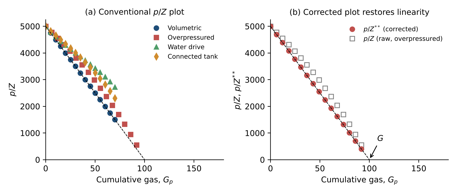Figure 2. (a) Typical p/Z signatures. (b) Applying the corrected $p/Z^{**}$ to overpressured data restores the straight line and the true $G$. Illustrative data.

3.3. Corrected (generalized) gas material balance

When additional drives are significant, the straight-line interpretation can be preserved by folding them into a modified compressibility factor. The approach follows King’s $p/Z^{*}$ for adsorbed gas and its extension to other mechanisms ($p/Z^{**}$, Moghadam et al.). The derivation below is a pore-volume budget for the gas zone.

3.3.1. Derivation

At pressure $p$, the space available to gas equals the original gas pore volume, $GB_{gi}$, less the volume lost to rock and water expansion and to net water influx. That space holds the gas still in the tank, including any gas received from a connected tank, $G_{\inf}$:

$$\begin{equation} \label{SMB-21} \left( G - G_{p} + G_{\inf} \right)B_{g} = GB_{gi}\left( 1 - \varepsilon_{fw} \right) - \left( W_{e} - W_{p} \right)B_{w}\tag{21} \end{equation}$$

Divide by $GB_{gi}$ and collect the non-gas terms into dimensionless fractions of the initial gas pore volume:

$$\begin{equation} \label{SMB-22} \omega_{w} = \frac{\left( W_{e} - W_{p} \right)B_{w}}{GB_{gi}},\quad\quad\omega_{g} = \frac{G_{\inf}B_{g}}{GB_{gi}}\tag{22} \end{equation}$$

$$\begin{equation} \label{SMB-23} \left( 1 - \frac{G_{p}}{G} \right)\frac{B_{g}}{B_{gi}} = 1 - \varepsilon_{fw} - \omega_{w} - \omega_{g}\tag{23} \end{equation}$$

With $B_{g}/B_{gi} = (Z/p)\left( p_{i}/Z_{i} \right)$ from Eq. (19):

$$\begin{equation} \label{SMB-24} \frac{p}{Z}\left( 1 - \varepsilon_{fw} - \omega_{w} - \omega_{g} \right) = \frac{p_{i}}{Z_{i}}\left( 1 - \frac{G_{p}}{G} \right)\tag{24} \end{equation}$$

Defining

$$\begin{equation} \label{SMB-25} Z^{**} = \frac{Z}{1 - \varepsilon_{fw} - \omega_{w} - \omega_{g}}\tag{25} \end{equation}$$

recovers the straight-line form:

$$\begin{equation} \label{SMB-26} \frac{p}{Z^{**}} = \frac{p_{i}}{Z_{i}}\left( 1 - \frac{G_{p}}{G} \right)\tag{26} \end{equation}$$

Each correction term is zero for the mechanism it represents when that mechanism is absent, so Eq. (26) collapses to Eq. (20) for a volumetric reservoir. Because $\omega_{w}$ and $\omega_{g}$ contain $G$, the solution is iterative: assume $G$, compute $Z^{**}$ at each survey, fit the line, update $G$, and repeat until the fitted and assumed values agree.

3.3.2. Overpressured reservoirs

In overpressured reservoirs gas compressibility at initial conditions is low enough to be comparable with rock and water compressibility. Ignoring $\varepsilon_{fw}$ produces the bowed trend in Figure 2a and an optimistic $G$ if early data are extrapolated. The rigorous expression for $\varepsilon_{fw}$ is Eq. (7); where residual oil or condensate occupies part of the pore space, a term $S_{or}\left\lbrack \exp\left( \int c_{o}\, dp' \right) - 1 \right\rbrack$ is added to its numerator. Pressure-dependent $c_{f}$ (common in unconsolidated or geopressured rock) is handled naturally by the integral form; the linear approximation, Eq. (8), is adequate only when $c_{f}$ is nearly constant.

3.3.3. Water-drive reservoirs

The term $\omega_{w}$ requires the cumulative water influx $W_{e}$, which is not measured and must be computed from an aquifer model (Section 3.4). The aquifer parameters are adjusted, together with $G$, until Eq. (26) is linear.

3.3.4. Connected reservoirs

The term $\omega_{g}$ requires the cumulative gas received from a second, unproduced tank of initial gas $G_{2}$. The second tank depletes volumetrically:

$$\begin{equation} \label{SMB-27} \frac{p_{2}}{Z_{2}} = \frac{p_{i}}{Z_{i}}\left( 1 - \frac{G_{\inf}}{G_{2}} \right)\tag{27} \end{equation}$$

and gas transfers between the tanks at a rate proportional to the pseudo-pressure difference:

$$\begin{equation} \label{SMB-28} q_{\inf} = \frac{dG_{\inf}}{dt} = J_{g}\left\lbrack m\left( p_{2} \right) - m(p) \right\rbrack,\quad\quad m(p) = 2\int_{p_{ref}}^{p}\frac{p'}{\mu Z}\, dp'\tag{28} \end{equation}$$

$G_{2}$ and the transfer coefficient $J_{g}$ are found by history-matching. Water drive and connected-tank behaviour can look alike on a $p/Z$ plot; the key difference is that water influx shrinks the gas pore volume while gas influx adds gas. A connected tank is indicated when the early $p/Z$ trend extrapolates to a $G$ smaller than the gas already produced, or when water production does not increase as a water-drive model would predict.

3.4. Aquifer models

3.4.1. Fetkovich pseudo-steady-state aquifer

A finite aquifer depletes according to its own material balance. With initial water volume $W_{i}$ and total aquifer compressibility $c_{t} = c_{w} + c_{f}$, the maximum encroachable water (aquifer pressure falling to zero) is

$$\begin{equation} \label{SMB-29} W_{ei} = c_{t}W_{i}p_{i}\tag{29} \end{equation}$$

The aquifer’s average pressure is therefore related to the cumulative influx by

$$\begin{equation} \label{SMB-30} {\bar{p}}_{a} = p_{i}\left( 1 - \frac{W_{e}}{W_{ei}} \right)\tag{30} \end{equation}$$

and, assuming pseudo-steady-state flow from aquifer to reservoir,

$$\begin{equation} \label{SMB-31} \frac{dW_{e}}{dt} = J_{w}\left( {\bar{p}}_{a} - p \right)\tag{31} \end{equation}$$

Differentiating Eq. (30) and substituting Eq. (31):

$$\begin{equation} \label{SMB-32} \frac{d{\bar{p}}_{a}}{dt} = - \frac{J_{w}p_{i}}{W_{ei}}\left( {\bar{p}}_{a} - p \right)\tag{32} \end{equation}$$

For a constant boundary pressure over an interval $\Delta t_{n}$, Eq. (32) integrates to an exponential decline of $\left( {\bar{p}}_{a} - p \right)$. Integrating Eq. (31) over the interval then gives the influx increment:

$$\begin{equation} \label{SMB-33} \Delta W_{e,n} = \frac{W_{ei}}{p_{i}}\left( {\bar{p}}_{a,n - 1} - {\bar{p}}_{n} \right)\left\lbrack 1 - \exp\left( - \frac{J_{w}p_{i}\,\Delta t_{n}}{W_{ei}} \right) \right\rbrack\tag{33} \end{equation}$$

where ${\bar{p}}_{n} = \left( p_{n - 1} + p_{n} \right)/2$ is the average boundary pressure over the step and ${\bar{p}}_{a,n - 1}$ is updated from Eq. (30) after each step. The two parameters, $W_{ei}$ and $J_{w}$, can be estimated from aquifer geometry and properties but are usually adjusted to match the pressure history. Unsteady-state models (van Everdingen–Hurst) may be used where infinite-acting aquifer behaviour must be represented more rigorously.

3.5. Limitations

• The $p/Z$ and $p/Z^{**}$ methods assume dry gas. For wet gas, convert produced condensate and water vapour to gas equivalent and add them to $G_{p}$. For gas condensates below the dew point, use a two-phase $Z$ factor or the generalized formulation of Section 5.
• Early-time data in overpressured or water-drive reservoirs carry little diagnostic power because the correction terms are still small; at least 10–20 % depletion is usually needed before the trend is reliable.

4. Oil Material Balance

The oil MBE contains more unknowns ($N$, $G$ or $m$, and aquifer parameters) than a single pressure survey can resolve. Instead of solving for $N$ at individual pressures, the recommended practice is to rearrange the equation into forms that plot as straight lines or that can be compared directly with measured pressures, and to use the departures as diagnostics.

4.1. Havlena–Odeh plot (all reservoir types)

Dividing Eq. (16) by the oil-zone expansion gives an equation of a straight line:

$$\begin{equation} \label{SMB-34} \underset{Y}{\underbrace{\frac{F - W_{e}B_{w}}{E_{o} + B_{oi}\,\varepsilon_{fw}}}} = N + G\,\underset{X}{\underbrace{\frac{B_{g} - B_{gi} + B_{gi}\,\varepsilon_{fw}}{E_{o} + B_{oi}\,\varepsilon_{fw}}}}\tag{34} \end{equation}$$

On a plot of $Y$ against $X$ (Figure 3) the intercept is the oil in place $N$ and the slope is the free (gas-cap) gas in place $G$. Water influx must be supplied from an aquifer model; if it is omitted when present, the points curve upward, which is itself a sign of water drive. The analyst can move the line in three ways:

• shift it vertically — changes $N$ with $G$ fixed;
• rotate about a point on the data — changes $N$ and $G$ together;
• rotate about the intercept — changes $G$ with $N$ fixed.

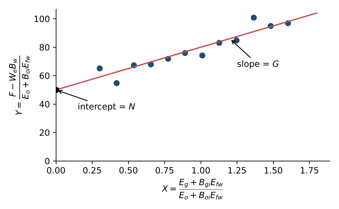Figure 3. Havlena–Odeh plot for a reservoir with a gas cap. The intercept gives $N$ and the slope gives $G$. Illustrative data.

Small pressure or PVT errors magnify scatter in $X$ and $Y$, especially early in depletion when the expansion terms are small. For an undersaturated oil the numerator of $X$ is zero, and the plot degenerates; use Section 4.2 instead.

4.2. F versus Et (no initial gas cap)

With no free gas initially ($m = 0$, $G = 0$), Eq. (15) reduces to

$$\begin{equation} \label{SMB-35} F - W_{e}B_{w} = N\left( E_{o} + E_{fw} \right) = NE_{t}\tag{35} \end{equation}$$

so the net withdrawal plotted against total expansion is a straight line through the origin with slope $N$ (Figure 4). The same plot is useful with a gas cap — with $E_{t} = E_{o} + mE_{g} + E_{fw}$ — as a consistency check of a proposed $(N,m)$ pair.

Shape	Interpretation
Straight line through origin	Model consistent: volumetric depletion, or all external drives correctly included.
Concave upward	Energy is missing from the model — unaccounted water influx, injection, a connected reservoir, or \(N\) (or \(m\)) too small.
Concave downward	The model contains too much energy — production from unmodelled wells, compressibility over-estimated, a declining influx, or \(N\) (or \(m\)) too large.
Isolated low point	Pressure not stabilized at the time of the survey, or a production or PVT error at that date.

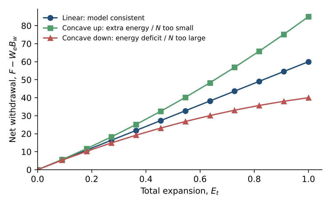Figure 4. F versus $E_{t}$ signatures. Illustrative data.

4.3. Water-drive form

When an aquifer is present and no gas cap exists, dividing Eq. (35) by $E_{t}$ gives

$$\begin{equation} \label{SMB-36} \frac{F}{E_{t}} = N + \frac{W_{e}B_{w}}{E_{t}}\tag{36} \end{equation}$$

With the correct aquifer model, $F/E_{t}$ versus $W_{e}B_{w}/E_{t}$ is a straight line of unit slope and intercept $N$. A slope other than one, or curvature, indicates that the aquifer size or strength is wrong.

4.4. Oil in place versus time

Solving Eq. (35) for $N$ at each survey,

$$\begin{equation} \label{SMB-37} N_{j} = \frac{F_{j} - W_{e,j}B_{w}}{E_{t,j}}\tag{37} \end{equation}$$

and plotting $N_{j}$ against time tests the assumed drive mechanism. A flat trend supports the model; a rising trend means energy is missing (aquifer, compaction, connected volume); a falling trend usually means not all producing wells are assigned to the reservoir. Because each point uses a single pressure, this plot is noisy and is best used as a supporting diagnostic.

4.5. Pressure diagnostics

Pressure versus cumulative oil and pressure versus time should be examined before any analysis. Typical features include:

• a change in slope at the bubble point, where liberated gas begins to supply energy and the decline slows;
• rising pressures marking the start of water or gas injection;
• flat pressures suggesting aquifer support (or, in tight reservoirs, that pressures are not yet representative of the drainage volume);
• outlying wells whose pressures do not follow the field trend and may not be in communication.

4.6. Pressure history match (synthetic pressure)

The most robust test of a material balance model is to compute the reservoir pressure it predicts and compare it with measurements. For trial values of $N$, $G$ and aquifer parameters, at each time $t_{n}$ solve for the pressure $p_{n}$ that satisfies the MBE:

$$\begin{equation} \label{SMB-38} R\left( p_{n} \right) = F\left( p_{n} \right) - N\left\lbrack E_{o}\left( p_{n} \right) + B_{oi}\,\varepsilon_{fw}\left( p_{n} \right) \right\rbrack - G\left\lbrack B_{g}\left( p_{n} \right) - B_{gi} + B_{gi}\,\varepsilon_{fw}\left( p_{n} \right) \right\rbrack - W_{e}\left( p_{n},t_{n} \right)B_{w} = 0\tag{38} \end{equation}$$

$F$ depends on $p_{n}$ through the PVT properties, and $W_{e}$ through the aquifer model, so $R\left( p_{n} \right) = 0$ is solved iteratively (for example by bisection or Newton’s method), marching forward in time. The calculated pressure history is then plotted against the measured static pressures (Figure 5).

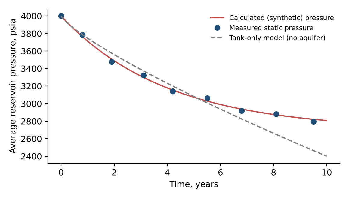Figure 5. Pressure history match. The tank-only model under-predicts pressure; adding an aquifer reproduces the measured trend. Illustrative data.

Working in pressure and time has practical advantages: the effect of shut-ins, rate changes, injection start-up and time-dependent influx is visible directly. A reliable workflow is:

1. Start with the simplest model (depletion only) and add mechanisms only when the match demands them.
2. Match from early to late time: initial pressure first, then early depletion, then late-time behaviour. Aquifer and connected-tank effects are small early and grow with time.
3. Recognize non-uniqueness — several combinations of $N$, $G$ and $W_{e}$ may match equally well; use volumetrics and other data to discriminate.

Poor early-time matches usually point to PVT errors, because the expansion terms are small and sensitive to $B_{o}$, $R_{s}$ and $B_{g}$. Isolated misfits point to bad pressures or production data at those dates.

4.7. Drive indices

Dividing the MBE by the hydrocarbon withdrawal $F_{hc} = N_{p}\left\lbrack B_{o} + \left( R_{p} - R_{s} \right)B_{g} \right\rbrack$ expresses each mechanism as a fraction of the total:

$$\begin{equation} \label{SMB-39} \underset{\text{DDI}}{\underbrace{\frac{NE_{o}}{F_{hc}}}} + \underset{\text{SDI}}{\underbrace{\frac{NmE_{g}}{F_{hc}}}} + \underset{\text{WDI}}{\underbrace{\frac{\left( W_{e} - W_{p} \right)B_{w}}{F_{hc}}}} + \underset{\text{CDI}}{\underbrace{\frac{NE_{fw}}{F_{hc}}}} + \underset{\text{IDI}}{\underbrace{\frac{W_{inj}B_{w} + G_{inj}B_{g,inj}}{F_{hc}}}} = 1\tag{39} \end{equation}$$

Index	Mechanism
DDI	Depletion (solution-gas) drive — expansion of oil and liberated gas
SDI	Segregation (gas-cap) drive
WDI	Natural water drive (net of produced water)
CDI	Compaction and connate-water expansion
IDI	Pressure maintenance by injection

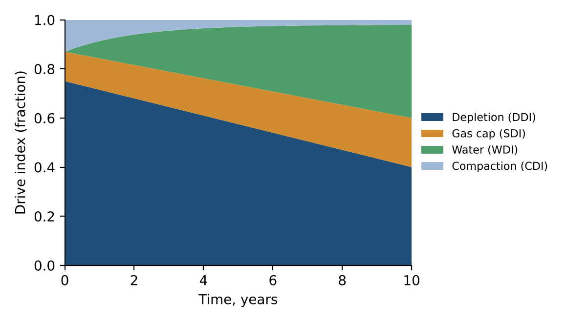Figure 6. Cumulative drive indices for a reservoir with a gas cap and a developing aquifer. Illustrative data.

Drive indices are cumulative and change with time (Figure 6). They provide a check on the solution: if the sum departs materially from unity — a practical tolerance is 0.95 to 1.05 — or trends steadily up or down, the MB solution is not consistent with the data. Common causes are mis-stated withdrawals or an incomplete set of energy terms.

4.8. Dake and Campbell diagnostic plots

Both plots assume a volumetric reservoir with no gas cap and look for departures from that assumption.

Dake plot. From Eq. (36), $F/E_{t} = N + W_{e}B_{w}/E_{t}$. Plotting $F/E_{t}$ (here $E_{t} = E_{o} + E_{fw}$, with constant $c_{f}$) against $N_{p}$ or time gives a horizontal line at $N$ for pure depletion. Any additional energy — water influx or an unrecognized gas cap — makes $F/E_{t}$ rise.

Campbell plot. $F/E_{t}$ is plotted against $F$, with $E_{t}$ including gas-cap expansion when one is present. Plotting against withdrawal rather than time makes the plot more sensitive to aquifer strength. Typical signatures are shown in Figure 7.

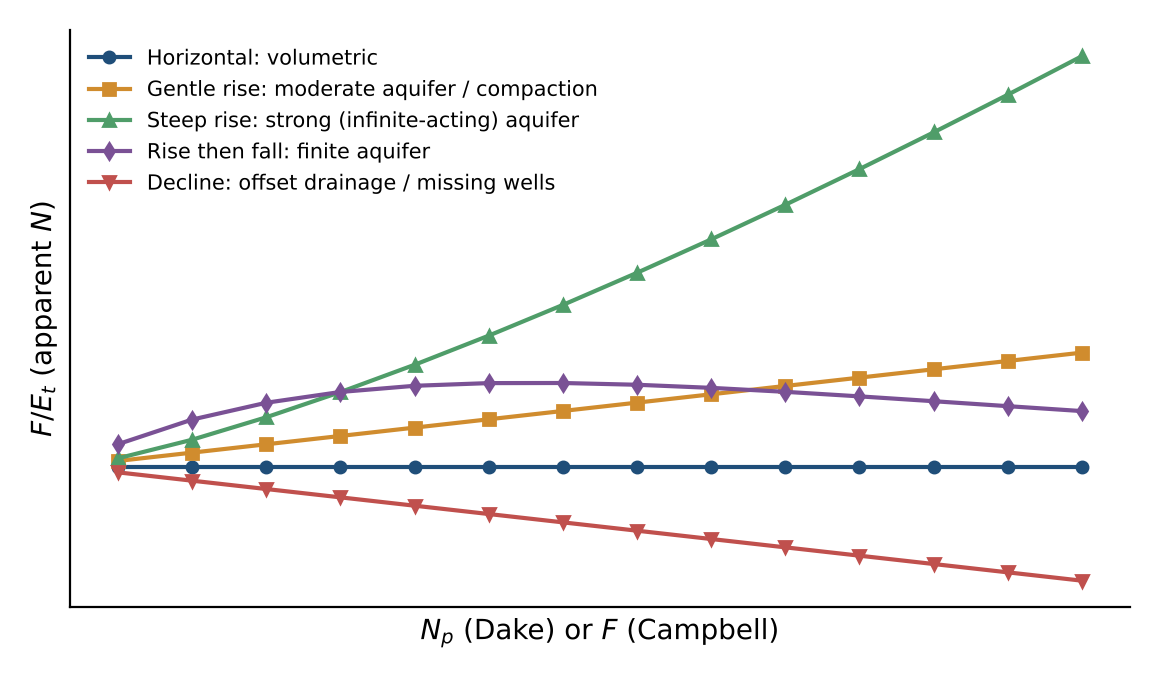Figure 7. Diagnostic signatures on Dake and Campbell plots.

Trend	Interpretation
Horizontal	Volumetric reservoir; energy from oil, solution gas and normal compaction only.
Gentle rise	Moderate water influx or abnormal pore compaction.
Steep, continuing rise	Strong, infinite-acting aquifer.
Rise then fall	Finite aquifer: support fades as the aquifer depletes.
Decline	Weak aquifer, or pressure lost to offset production or unassigned wells.

These plots, like the $N$-versus-time plot, are qualitative. When pressure surveys are infrequent, trends may not be identifiable.

5. Volatile Oil and Gas Condensate (Generalized MBE)

Conventional black-oil MB assumes the gas phase carries no liquid. In volatile oils (typically $R_{si} > 500$ scf/STB, API gravity above about 40°) and gas condensates, the free gas contains significant vaporized oil, described by the solution oil–gas ratio $R_{v}$ (STB/scf). Ignoring $R_{v}$ overstates oil recovery from the oil zone and misallocates surface gas and oil between phases.

The generalized MBE (Walsh) tracks stock-tank oil and surface gas in both reservoir phases. Let $N_{foi}$ be the oil initially in the free-oil phase and $G_{fgi}$ the gas initially in the free-gas phase. The totals are

$$\begin{equation} \label{SMB-40} N = N_{foi} + G_{fgi}R_{vi},\quad\quad G = G_{fgi} + N_{foi}R_{si}\tag{40} \end{equation}$$

Withdrawal is converted to reservoir volumes by splitting surface production back into reservoir oil and gas phases:

$$\begin{equation} \label{SMB-41} F = \frac{N_{p}\left( B_{o} - R_{s}B_{g} \right) + G_{p}\left( B_{g} - R_{v}B_{o} \right)}{1 - R_{v}R_{s}} + \left( W_{p} - W_{inj} \right)B_{w} - G_{inj}B_{g,inj}\tag{41} \end{equation}$$

The oil- and gas-phase expansivities become

$$\begin{equation} \label{SMB-42} E_{o} = \frac{B_{o}\left( 1 - R_{v}R_{si} \right) + B_{g}\left( R_{si} - R_{s} \right)}{1 - R_{v}R_{s}} - B_{oi}\tag{42} \end{equation}$$

$$\begin{equation} \label{SMB-43} E_{g} = \frac{B_{g}\left( 1 - R_{s}R_{vi} \right) + B_{o}\left( R_{vi} - R_{v} \right)}{1 - R_{v}R_{s}} - B_{gi}\tag{43} \end{equation}$$

and the balance, analogous to Eq. (16), is

$$\begin{equation} \label{SMB-44} F - W_{e}B_{w} = N_{foi}\left( E_{o} + B_{oi}\,\varepsilon_{fw} \right) + G_{fgi}\left( E_{g} + B_{gi}\,\varepsilon_{fw} \right)\tag{44} \end{equation}$$

Setting $R_{v} = R_{vi} = 0$ recovers the black-oil forms: Eq. (41) becomes Eq. (10), Eq. (42) becomes Eq. (12), and $E_{g}$ becomes $B_{g} - B_{gi}$. All plots in Section 4 apply unchanged with these definitions; for example, the Havlena–Odeh intercept and slope now give $N_{foi}$ and $G_{fgi}$, from which $N$ and $G$ follow through Eq. (40). For a gas condensate with no initial oil phase, $N_{foi} = 0$ and Eq. (44) yields $G_{fgi}$ directly.

6. Recommended Workflow

1. Assemble and check data. Reconcile production and injection volumes by well; correct pressures to datum; validate PVT (consistency of $B_{o}$, $R_{s}$, $B_{g}$ at the bubble point; $R_{v}$ for volatile systems).
2. Inspect pressure trends against time and cumulative production to identify the bubble point, injection start, aquifer support and anomalous wells.
3. Select the reservoir type — gas or oil; gas cap or not; volatile or black oil.
4. Apply the simplest model. For gas, the $p/Z$ plot; for oil, F versus $E_{t}$ or Havlena–Odeh.
5. Diagnose departures using the shape of the primary plot, $N$ versus time, and Dake or Campbell plots.
6. Add mechanisms only as needed — compaction (rigorous $\varepsilon_{fw}$), aquifer, connected tank — and refine with the $p/Z^{**}$ or pressure history match.
7. Validate the solution. Drive indices should sum to about one; the synthetic pressure should match measured pressures; $N$ and $G$ should be consistent with volumetric estimates.
8. Document non-uniqueness by reporting the range of solutions that match equally well.

Nomenclature

Symbol	Description	Field units
$B_{g}$	Gas formation volume factor	rb/scf
$B_{o}$	Oil formation volume factor	rb/STB
$B_{w}$	Water formation volume factor	rb/STB
$c_{e}$	Effective oil-zone compressibility	psi⁻¹
$c_{f}$	Pore-volume (formation) compressibility	psi⁻¹
$c_{o}$, $c_{w}$	Oil and water compressibility	psi⁻¹
$E_{o}$	Oil plus dissolved-gas expansion	rb/STB
$E_{g}$	Gas-cap expansion (per STB, Eq. 13; per scf, Eq. 43)	rb/STB, rb/scf
$E_{fw}$	Connate-water and pore-volume expansion	rb/STB
$E_{t}$	Total expansion	rb/STB
$\varepsilon_{fw}$	Fractional HCPV reduction from rock and water expansion	–
$F$	Net underground withdrawal	rb
$G$	Original free gas in place	scf
$G_{\inf}$	Cumulative gas influx from a connected tank	scf
$J_{w}$, $J_{g}$	Aquifer and inter-tank transfer coefficients	STB/d/psi; scf/d/(psi²/cp)
$m$	Initial gas-cap to oil-zone volume ratio	–
$m(p)$	Real-gas pseudo-pressure	psi²/cp
$N$	Original oil in place	STB
$p$, $p_{i}$	Average and initial reservoir pressure	psia
$R_{p}$	Cumulative produced gas–oil ratio	scf/STB
$R_{s}$	Solution gas–oil ratio	scf/STB
$R_{v}$	Solution oil–gas ratio (vaporized oil)	STB/scf
$S_{wi}$	Initial water saturation	fraction
$T$	Reservoir temperature	°R
$W_{e}$	Cumulative water influx	STB
$W_{ei}$	Maximum encroachable water (Fetkovich)	STB
$Z$, $Z^{**}$	Gas deviation factor and corrected deviation factor	–
$\omega_{w}$, $\omega_{g}$	Water- and gas-influx fractions of initial gas pore volume	–

References

1. Dake, L.P. 1978. Fundamentals of Reservoir Engineering. Amsterdam: Elsevier.
2. Walsh, M.P. and Lake, L.W. 2003. A Generalized Approach to Primary Hydrocarbon Recovery. Amsterdam: Elsevier.
3. Schilthuis, R.J. 1936. Active Oil and Reservoir Energy. Trans. AIME 118: 33–52.
4. Havlena, D. and Odeh, A.S. 1963. The Material Balance as an Equation of a Straight Line. J. Pet. Tech. 15 (8): 896–900.
5. Fetkovich, M.J. 1971. A Simplified Approach to Water Influx Calculations — Finite Aquifer Systems. J. Pet. Tech. 23 (7): 814–828.
6. van Everdingen, A.F. and Hurst, W. 1949. The Application of the Laplace Transformation to Flow Problems in Reservoirs. Trans. AIME 186: 305–324.
7. Campbell, R.A. and Campbell, J.M. 1978. Mineral Property Economics, Vol. 3: Petroleum Property Evaluation. Norman, Oklahoma: Campbell Petroleum Series.
8. King, G.R. 1993. Material-Balance Techniques for Coal-Seam and Devonian Shale Gas Reservoirs With Limited Water Influx. SPE Res. Eng. 8 (1): 67–72.
9. Moghadam, S., Jeje, O. and Mattar, L. 2011. Advanced Gas Material Balance in Simplified Format. J. Can. Pet. Tech. 50 (1): 90–98.
10. Walsh, M.P., Ansah, J. and Raghavan, R. 1994. The New, Generalized Material Balance as an Equation of a Straight Line: Part 1 — Applications to Undersaturated and Volumetric Reservoirs; Part 2 — Applications to Saturated and Non-Volumetric Reservoirs. SPE 27684 and SPE 27728.