Separator data
Example: Working with Separator Data
Separator data can be tricky to work with, so in this section we'll focus on how you can efficiently work with and handle separator rates in whitson+. Learn the most important things in less than 30 minutes.
Info
The examples shown in the videos below use the "Default EOS option" in whitson+ (more info here). Hence, if you are using a custom EOS, your results will be slighly different for the rest of these examples. However, the main objective of this is to learn the practicalities of the software, so it's not important in this context.
1.1 Fluid Definition with Separator Data
- In the Wells module, click ADD WELL up to the right.
- Add well with name for example: Separator Data Example.
- Click SAVE.
- Download the relevant data here.
- Go to the PVT module in the navigation panel.
- Open the Reservoir Fluid Composition Input Card.
- Change the Method from "GOR" to "Separator Compositions".
- Copy the right data from The Excel Sheet and paste it into the relevant cells.
- Click HOFFMAN QC:
- NB:The blue dots overlay the grey line, indicating the separator oil and gas compositions are in equilibrium. Occasionally, there may be significant differences in Nitrogen due to its small quantities, but it can be ignored. The most important is that the majority of C1 to C6 is on the line, also the C7+ is decent.
- Read more about HOFFMAN QC here.
- Click SAVE.
- Check the predicted fluid composition by clicking the "eye icon".
- Check the black oil table.
- All steps are shown in the .gif above.
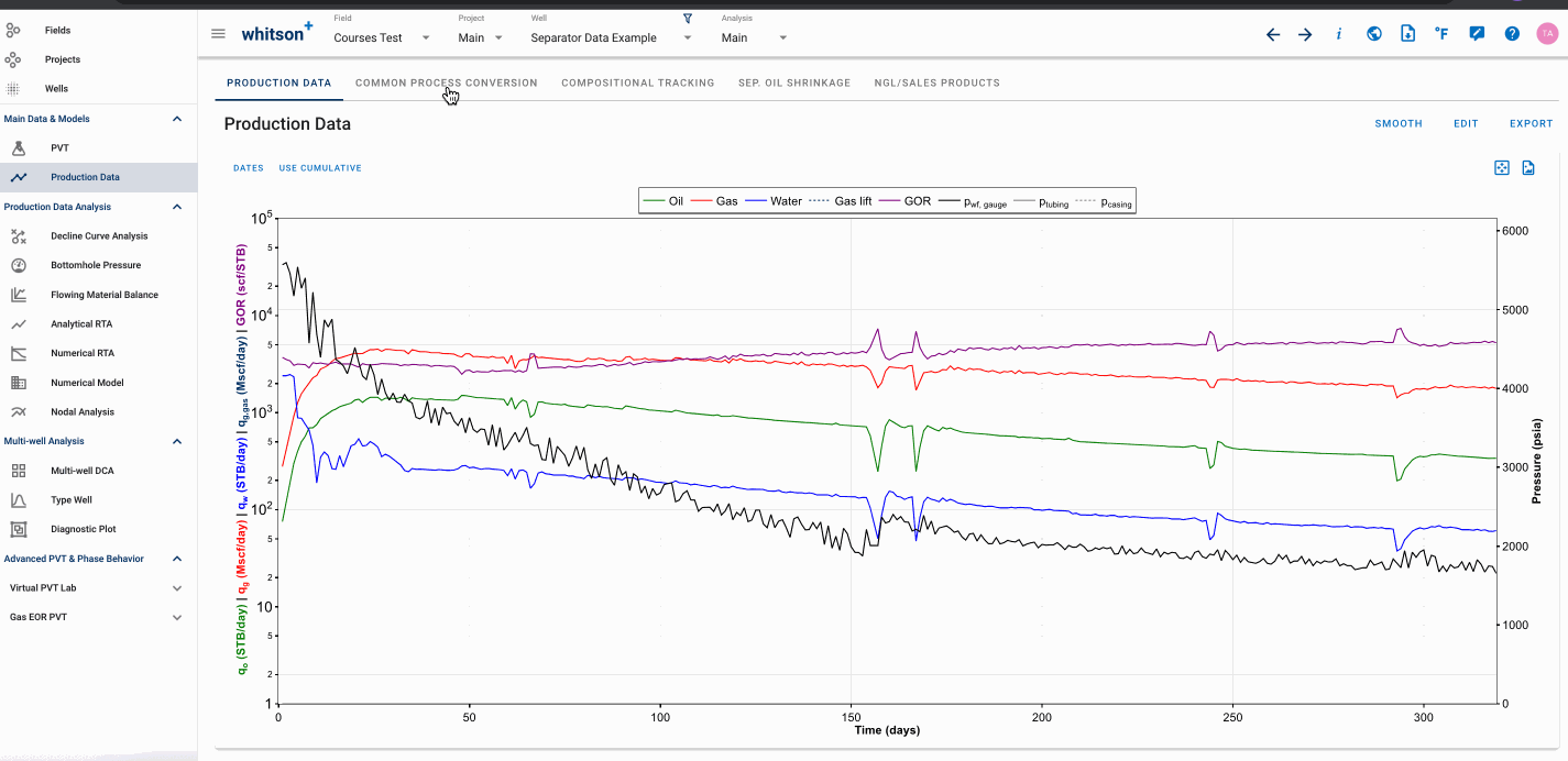
1.2 Upload Production Data -Rates Measured at Separator Conditions
- Download the relevant data here.
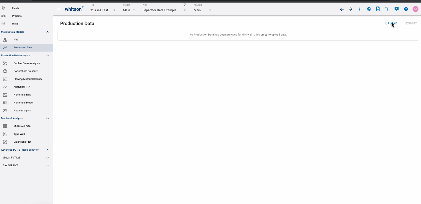
- Go to the Production Data module.
- Click UPLOAD up to the right.
- Select the DATADUMP.
- Drop the data file into the DATADUMP box in the front end.
- Click SAVE.
- Click EDIT.
- Change the Rate Input from Stock Tank Rates into Separator Rates (Common Process).
- Click SAVE.
- You’ll get the prompt "Calculation of Common Process Rates will be launched".
- Click YES.
- All steps are shown in the .gif above.
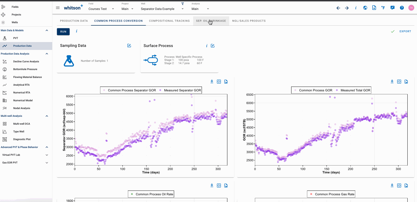
1.3 Common Process Conversion
- In the Production Data module.
- Click on the Common Process Conversion tab.
- The calculation is automatically done upon uploading the separator rates, but you can rerun if some changes have been made and are not reflected in the common process rate.
- All steps are shown in the .gif above.
- Read more about Common Process Conversion here.
1.4 Separator Oil Shrinkage Calculations
- In the Production Data module.
- Click on the Sep. OIL SHRINKAGE tab.
- The calculation is automatically done upon uploading the separator rates, but you can rerun if some changes have been made and are not reflected in the common process rate.
- Check Separator Oil Shrinkage Calculations.
- All steps are shown in the .gif above.
- Read more about Separator Oil Shrinkage here.
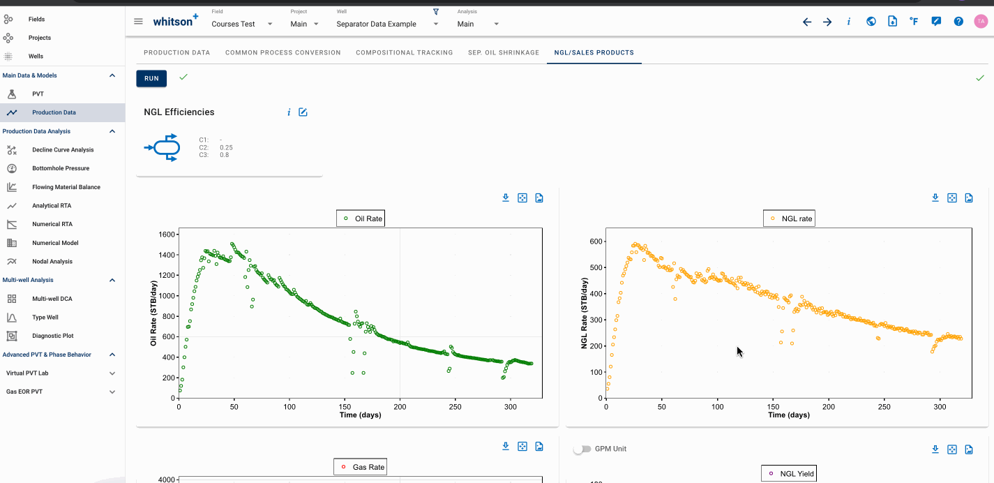
1.5 Sales Products - NGL Yield vs Time
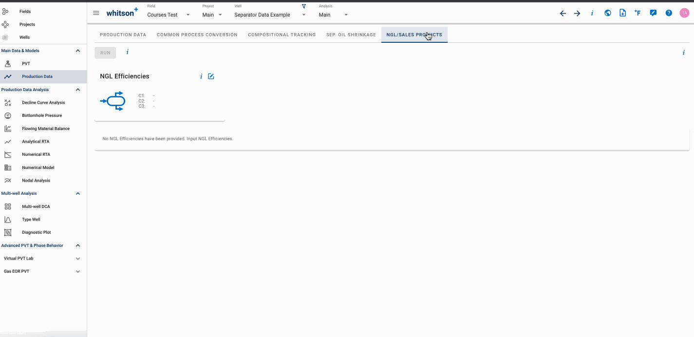
- In the Production Data module.
- Click the NGL/SALES PRODUCTS tab up to the right.
- Open the NGL Efficiencies input card.
- Change the NGL Recovery Method to the Dewpoint Control.
- Click SAVE.
- Click RUN.
- All steps are shown in the .gif above.
- Read more about Sales Products - NGL calculation here.
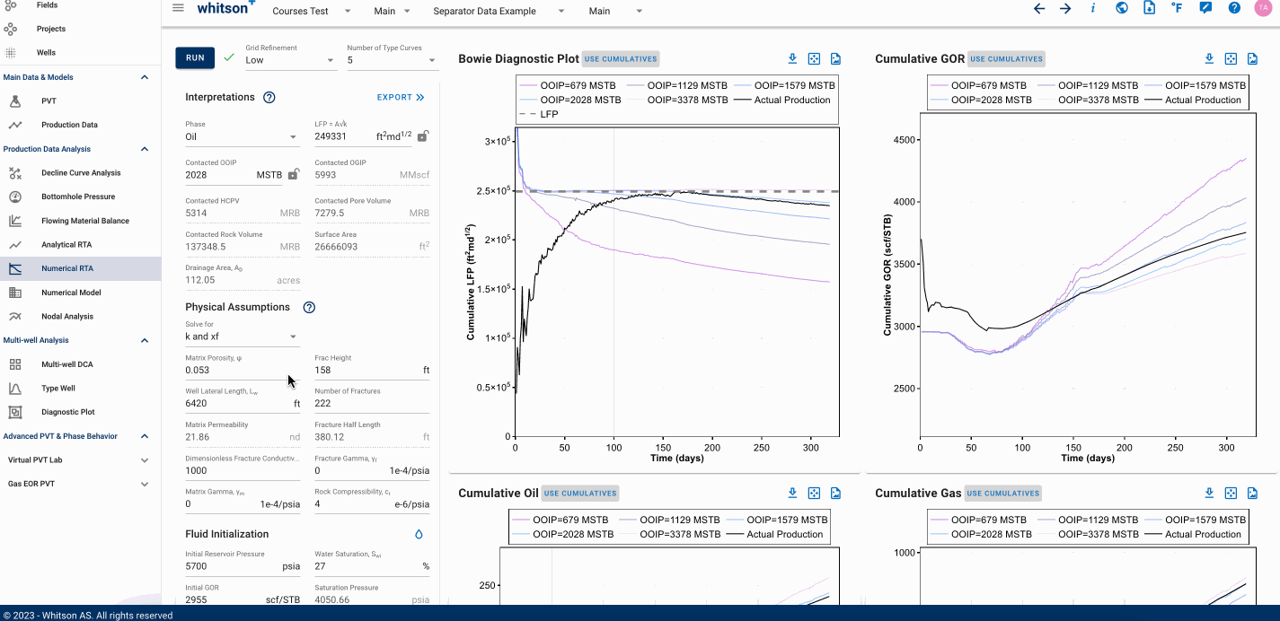
1.6 Numerical RTA
In the Numerical RTA module.
- First RUN: Default values.
- Click RUN.
- This run will give us the initial simulation with the default input values.
- Second RUN: we can proceed to adjust the values as per the data provided in the Excel sheet here:
- Provide the relevant Fluid Initialization data.
- Provide the relevant Well data.
- Open the Relative Permeability input card, provide the relevant Relative Permeability data and click save.
- Click RUN, this second run should give you a much better match of the GORs and water cuts (you may adjust the relative permeabilities further if you want).
- All steps are shown in the .gif above.
Info
You will only need to re-run (click RUN) the numerical RTA module when you update any of the following parameters: PVT, Swi, Fcd, relative permeability, pressure-dependent permeability (gamma matrix/fracture) or initial pressure.
1.7 Numerical Model
- To transfer the results from the Numerical RTA module into the numerical model, click EXPORT at the top of the Interpretation menu in the Numerical RTA module.
- Read the pop-up box text and click YES. This exports the results into the Numerical Model.
- In the numerical model, click RUN
- All steps are shown in the .gif above.