PTA - Pressure Transient Analysis

Purpose of Well Testing

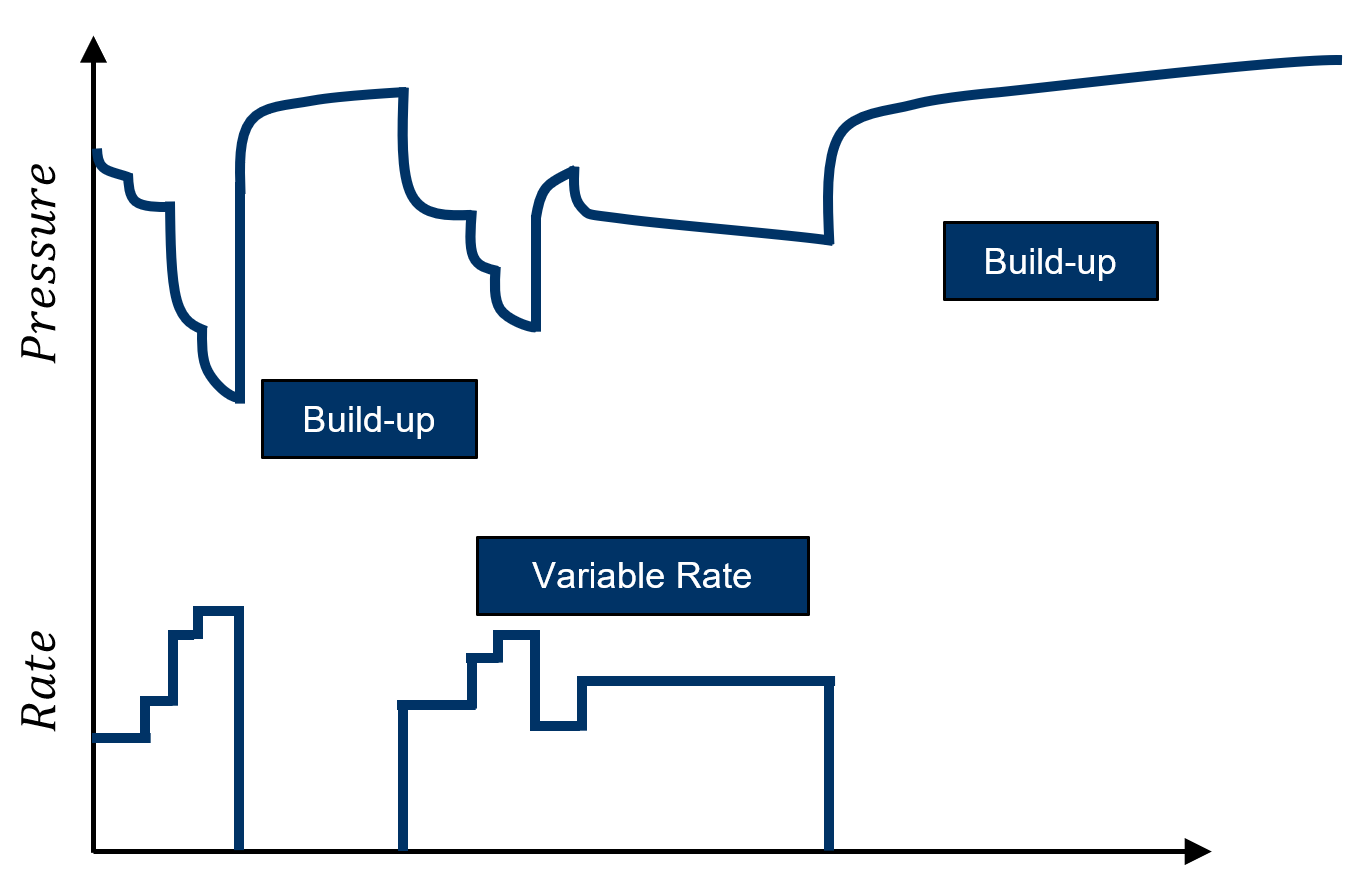
Well testing is a fundamental tool in reservoir engineering, used to gain insight into the dynamic behavior of subsurface formations. A well test involves measuring the pressure response of a well to a controlled and defined change in operating conditions, typically a change in flow rate. In most conventional applications, the flow rate is maintained at a specified value while bottomhole pressure is recorded; however, alternative testing approaches also exist. The selection of the appropriate test type depends on factors such as the timing of the test, well location, reservoir and fluid properties, operational costs, and the value of the information to be obtained. Each well test methodology is associated with its own analytical framework, including characteristic equations and diagnostic plots, to support interpretation of the acquired data.

A drawdown test is performed by producing the well at a constant flow rate or a defined sequence of rates while recording the corresponding pressure decline over time. Drawdown data quality can be adversely affected by rate fluctuations, making the pressure derivative more susceptible to noise. These tests are typically considered when minimizing production downtime is a priority, such as under economic or operational constraints.

A buildup test is conducted by producing the well at a constant rate for a sufficient period, followed by a shut-in during which the pressure recovery is measured. The pre-shut-in flow period should be long enough to stabilize the flow regime, ensuring that transient behavior reflects reservoir properties rather than wellbore storage or operational disturbances. Because there is no flow during shut-in, buildup data generally exhibits lower noise levels and yields more reliable derivative responses compared to drawdown tests. When interpreting buildup data, it is good practice to evaluate the preceding drawdown period as well, since the combined dataset can enhance diagnostic and model-matching accuracy.

Injection and fall-off tests are the direct analogs of drawdown and buildup tests, but applied to injection wells. In an injection test, fluid is introduced into the reservoir at a controlled rate while bottomhole pressure is monitored. The injection period is analogous to a drawdown in a production well, except that the direction of flow is reversed. Following injection, the well is shut in, and the fall-off period records the pressure decline over time, which is equivalent to a buildup in production testing. These tests are widely used in waterflood injectors, disposal wells, and gas storage projects.

Well test interpretation is, by nature, an inverse problem. In this context, the measured inputs are the flow rate history and the corresponding pressure response, while the unknown is the underlying reservoir model and its parameters. The interpretation process must solve two distinct but interconnected tasks:

1. Model identification – determining the most appropriate conceptual model of the reservoir–wellbore system, including flow geometry, boundary conditions, and any wellbore effects.

2. Parameter estimation – quantifying key reservoir and wellbore properties, such as permeability, skin factor, storativity, and boundary location, based on the identified model.

Well Test Interpretation

Quantitative well test interpretation commonly employs three main approaches: straight-line analysis, type-curve analysis, and simulation/history matching. Each has distinct strengths and limitations, and selection depends on the objectives, available data, and desired level of precision.

Straight-line methods are widely used in well test interpretation to identify flow regimes from transformed pressure and time data. From the slope and intercept of straight-line trends, it is possible to estimate reservoir or fracture properties such as permeability, skin factor, and, in multi-fractured horizontal wells (MFHW), fracture conductivity or half-length. These methods are straightforward to apply and yield reliable results when distinct flow regimes are present.

Type-curve methods compare field data to theoretical type curves derived from idealized reservoir models. They honor more of the dataset and are less prone to inconsistencies but can be more time-consuming and require specialized matching tools.

Simulation and history matching use analytical or numerical models to reproduce the observed pressure response, adjusting unknown parameters until a match is achieved. This approach can incorporate more complex reservoir and wellbore behaviors, but it is computationally intensive and requires good initial parameter estimates.

Mathematical Formulation of Flow Equations for Well Test Interpretation

An understanding of fluid flow in porous media is central to well test interpretation, as it explains how pressure disturbances propagate through the reservoir. The diffusivity equation describes the transient movement of a slightly compressible fluid through a porous medium. Its derivation combines three fundamental principles of fluid flow in reservoirs: the continuity equation, and the equation of state for a slightly compressible liquid and Darcy’s law under a set of simplifying assumptions:

• The reservoir contains a single-phase fluid, and multiphase flow effects (e.g., gas–oil or water–oil flow) are not present.

• The fluid is slightly compressible.

• Flow in the reservoir obeys Darcy’s law

• Rock and fluid properties, including porosity ($ϕ$), permeability ($k$), viscosity ($μ$), and total compressibility ($c_t$), remain constant throughout the analysis.

The continuity equation expresses the principle of mass conservation for fluid flow in porous media. It relates the net rate of mass entering an infinitesimal control volume to the rate of mass accumulation within that volume. For one-dimensional linear flow, it can be written as:

$$\begin{equation} \frac{\partial}{\partial x}(\rho u_x) = -\frac{\partial}{\partial t}(\rho \phi) \end{equation}$$

Where the superficial velocity, $u_x$, is defined as the volumetric flow rate per unit cross-sectional area.

The equation of state for a slightly compressible liquid defines compressibility as the fractional change in volume per unit change in pressure, expressed as:

$$\begin{equation} c = \frac{1}{\rho}\left(\frac{d\rho}{dp}\right)_T = -\frac{1}{V}\left(\frac{dV}{dp}\right)_T \end{equation}$$

and assumed constant over the pressure range of interest. This is a valid approximation for single-phase oil or water systems and may also be applied to gas flow when drawdown is small enough that fluid properties remain nearly constant.

Darcy’s law describes fluid motion through a porous medium resulting from a pressure gradient. It states that, for steady, incompressible, single-phase flow, the volumetric flow rate is proportional to the pressure drop across the medium and to the cross-sectional area of flow, and inversely proportional to fluid viscosity and flow length. In one-dimensional form, the superficial velocity can be expressed as:

$$\begin{equation} u_x = -\frac{k}{\mu} \frac{dp}{dx} \end{equation}$$

The diffusivity equation is obtained by combining three fundamental relationships. This formulation describes transient fluid flow in porous media, linking the spatial variation of pressure to its change over time through rock and fluid properties.

For one-dimensional linear flow, the diffusivity equation can be expressed as:

$$\begin{equation} \frac{\partial^2 p}{\partial x^2} = \frac{\phi \mu c_t}{k} \frac{\partial p}{\partial t} \end{equation}$$

In radial coordinates,

$$\begin{equation} \frac{1}{r}\frac{\partial}{\partial r}\left(r\frac{\partial p}{\partial r}\right) = \frac{\phi \mu c_t}{k}\frac{\partial p}{\partial t} \end{equation}$$

The diffusivity equation is a linear partial differential equation that is first order with respect to time and second order with respect to spatial coordinates. To obtain a solution, the equation must be solved in conjunction with appropriate initial conditions (IC), which define the pressure distribution at the start of the analysis, and boundary conditions (BC), which specify the pressure or flow behavior at the reservoir boundaries or at the wellbore. When these conditions are applied, the solution provides pressure distribution as a function of spatial position and time, $p = p(r,t)$ , enabling the prediction of reservoir response under specified operating scenarios.

Infinite-Acting Radial Flow

One of the primary analytical solutions to the radial diffusivity equation describes infinite-acting radial flow (IARF) in a homogeneous, laterally extensive reservoir with uniform initial pressure. The solution assumes an infinitesimal line-source well producing at a constant rate. Under these conditions, the pressure at any radial distance r and time t can be expressed (in oilfield units) as:

$$\begin{equation} p(r,t) = p_i + \frac{70.6qB\mu}{kh} \text{Ei}\left(-\frac{948\phi\mu c_t r^2}{kt}\right) \end{equation}$$

Where,

$$\begin{equation} \text{Ei}(-x) = \int_{x}^{\infty} \frac{e^{-y}}{y} \,dy \end{equation}$$

Where $p_i$ is the initial reservoir pressure in psia, $q$ is the production rate in STB/D, $B$ is the formation volume factor in RB/STB, $μ$ is viscosity in cp, $k$ is permeability in md, $h$ is formation thickness in feet, $ϕ$ is porosity, $c_t$​ is total compressibility in $psi^{-1}$, and $t$ is time in hours.

Logarithmic Approximation

When the dimensionless argument,

$$\begin{equation*} \frac{948 \phi \mu c_t r^2}{k t} \end{equation*}$$

is less than 0.02, the exponential integral function $Ei(-x)$ can be approximated by the logarithmic expression,

$$\begin{equation*} \text{Ei}(-x) \approx \ln(1.781 x) \end{equation*}$$

Under this condition, the infinite-acting radial flow solution can be rewritten without the exponential integral term, yielding:

$$\begin{equation} p(r,t) = p_i - \frac{162.6 \mu B}{kh} \left[\log\left(\frac{kt}{\phi\mu c_t r^2}\right) - 3.23\right] \end{equation}$$

This form is particularly useful for early-time analysis when the dimensionless time is large enough that the logarithmic approximation remains valid, simplifying computations in well test interpretation.

As an example, when estimating pressure at the wellbore during transient flow, the logarithmic approximation can be applied in the following form:

$$\begin{equation} p_{wf} = p_i - 162.6\frac{qB\mu}{kh}\left(\log t + \log\frac{k}{\phi\mu c_t r_w^2} - 3.2274\right) \end{equation}$$

Wellbore and Near-Wellbore Phenomena in Well Testing

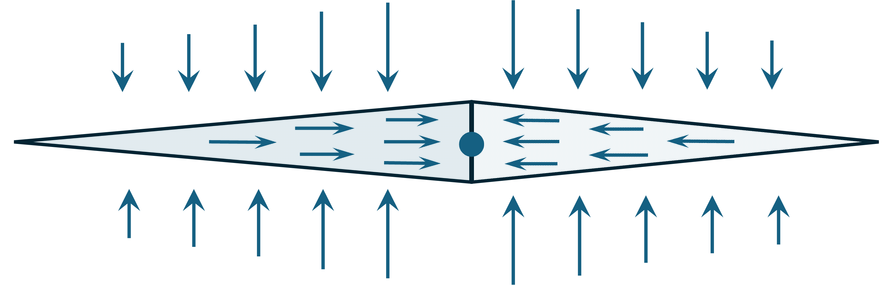
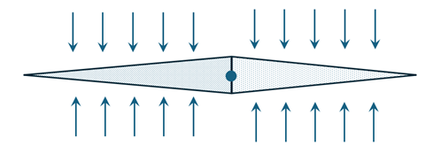
In pressure transient analysis, certain near-wellbore phenomena can significantly influence the early-time portion of the pressure response and must be accounted for to accurately determine reservoir properties. Two of the most common effects are skin and wellbore storage. The skin factor quantifies additional pressure drop or gain near the wellbore caused by formation damage, stimulation, or altered permeability zones, while wellbore storage represents the temporary storage or release of fluids within the wellbore itself as the system responds to a change in flow conditions. Both effects can mask or distort the true reservoir response if not properly recognized and corrected during interpretation. Understanding these mechanisms is essential for separating wellbore influences from reservoir behavior and for ensuring that derived parameters, such as permeability and boundary characteristics, are reliable.

Related concepts, such as skin factor, and wellbore storage, enhance the ability to interpret pressure transients and characterize reservoir properties.

Near-Wellbore Permeability Alteration: Damage and Stimulation

In deriving the infinite-acting radial flow solution, it is typically assumed that the well is vertical, fully penetrates the productive interval, and has not been subjected to damage or stimulation. In practice, however, the near-wellbore region may be altered by factors such as drilling-induced damage, partial completion, perforating, gravel packing, or stimulation treatments. These effects are often quantified using a single dimensionless parameter known as the skin factor. The skin factor represents the additional pressure drop (or gain) at the wellbore relative to that predicted for an undamaged well under otherwise identical conditions.

A practical way to model damage or stimulation is to treat the near-wellbore alteration as a cylindrical shell of uniform permeability $k_a$​ extending from the wellbore radius $r_w$​ to an outer radius $r_a$​. Outside this altered zone, the formation permeability remains equal to the original reservoir value. When $k_a$ is less than $k$, the zone impedes flow and the well is considered damaged. When $k_a$​ exceeds $k$, the well is considered stimulated.

In the absence of any alteration, the pressure drop across the near-wellbore region can be expressed as:

$$\begin{equation} \Delta p = \frac{141.2 q B \mu}{k h} \ln\left(\frac{r_a}{r_w}\right) \end{equation}$$

If the altered zone is present, the pressure drop is instead:

$$\begin{equation} \Delta p_d = \frac{141.2 q B \mu}{k_a h} \ln\left(\frac{r_a}{r_w}\right) \end{equation}$$

Comparing these two cases allows calculation of the skin factor, which quantifies the impact of near-wellbore permeability alteration on well performance.

Quantifying Additional Pressure Drop from Altered Permeability

The incremental pressure drop caused by a damaged or stimulated zone can be obtained by comparing the near-wellbore pressure losses for the altered and unaltered cases.

$$\begin{equation} \Delta P_{skin} = Pwf_{ideal} - Pwf_{obs} \end{equation}$$

The additional pressure drop due to the altered zone is obtained by subtracting the bottomhole pressure for the undisturbed permeability case from that of the altered zone case:

$$\begin{equation} \Delta p_s = \frac{141.2 q B \mu}{k h}\left(\frac{k}{k_a} - 1\right)\ln\left(\frac{r_a}{r_w}\right) \end{equation}$$

Following the formulation introduced by Hawkins (1956), the dimensionless skin factor, $s$, is defined as:

$$\begin{equation} s = \left(\frac{k}{k_a} - 1\right)\ln\left(\frac{r_a}{r_w}\right) \end{equation}$$

This parameter allows the additional pressure drop to be written in a compact form:

$$\begin{equation} \Delta p_s = \frac{141.2 q B \mu}{k h} s \end{equation}$$

The skin factor can also be expressed in terms of an effective wellbore radius, which represents the radius of an ideal, undamaged wellbore that would yield the same productivity as the actual well. This relationship is given by:

$$\begin{equation} r_{\text{eff}} = r_w e^{-s} \end{equation}$$

The flowing pressure at the wellbore can be determined by evaluating the radial diffusivity solution (Eq. 8) at $r = rw​$ and incorporating the additional drawdown associated with the skin factor as defined in Eq. 15. This approach accounts for both the reservoir flow behavior and the near-wellbore pressure losses (or gains) caused by formation damage or stimulation:

$$\begin{equation} p_{wf} = p_i - 162.6\frac{qB\mu}{kh}\left(\log t + \log\frac{k}{\phi\mu c_t r_w^2} - 3.2274 + 0.8686s\right) \end{equation}$$

Eq.17 provides the fundamental relationship used in conventional semi-log straight-line methods for interpreting drawdown and buildup tests.

Infinite-Acting Radial Flow: Fundamentals and Interpretation

Infinite-acting radial flow (IARF) is one of the most frequently observed flow regimes in PTA and serves as the basis for many diagnostic and interpretation techniques. Under IARF conditions, the transient pressure response exhibits a linear relationship with the logarithm of elapsed time, a feature that enables the application of straight-line analysis methods for parameter estimation.

Drawdown Tests

From a theoretical perspective, the constant-rate drawdown test is the simplest to analyze, as it closely matches the constant terminal rate boundary condition commonly assumed in the derivation of classical analytical well test solutions. In this test type, the well is initially shut in, with reservoir pressure uniform across the drainage area. Production is then initiated at a fixed surface or sandface rate $q​$, and the flowing bottomhole pressure, $p_{wf}​$,​ is measured over time as the reservoir pressure declines.

During the infinite-acting radial flow period, a plot of bottomhole flowing pressure, $p_{wf}​$​, versus the logarithm of elapsed time produces a straight-line trend. The slope of this trend is proportional to the reciprocal of formation transmissibility and can be used to calculate permeability.

$$\begin{equation} m = 162.6\frac{qB\mu}{kh} \end{equation}$$

Many conventional well test interpretation methods rely on the semi-log analysis approach, where the identification of a linear trend on a semi-logarithmic plot of pressure versus time is essential. Correctly recognizing and selecting the appropriate semi-log straight line is a key step in this process, as it directly influences the accuracy of permeability–thickness ($kh​$) estimates and other derived reservoir parameters.

The intercept $b​$, expressed in Eq. ???, corresponds to the extrapolated bottomhole pressure at $t = 1​$ hour, incorporating formation properties, well geometry, and the dimensionless skin factor, $s​$. This intercept is essential for determining skin and diagnosing wellbore damage or stimulation effectiveness.

$$\begin{equation} s = 1.151\left[\frac{p_i - p_{1hr}}{m} - \log\frac{k}{\phi\mu c_t r_w^2} + 3.2274\right] \end{equation}$$

When determining $p_{1hr}​$​, the value should be obtained from the extrapolated straight-line trend on the semi-log plot rather than taken directly from the measured pressure at one hour. Using the measured pressure at that point could introduce error, whereas extrapolation from the established straight line ensures consistency with the underlying model assumptions.

In field operations, it is often challenging to maintain an exact constant production rate throughout a drawdown test. Even minor deviations from the target rate can significantly affect the interpretation when using constant-rate analytical models. To demonstrate this sensitivity, consider a test in which the flow rate gradually decreases by approximately 10% over the test duration. The corresponding pressure response shows an upward trend toward the end of the test, indicating that the pressure decline rate is no longer consistent with infinite-acting radial flow under constant-rate conditions.

If such late-time data were analyzed under the assumption of a perfectly constant flow rate, the calculated slope of the semi-log straight line could yield an unrealistic result. In extreme cases, the algebraic sign of the slope may reverse, producing a negative permeability estimate—an indication that the constant-rate assumption has been violated.

$$\begin{equation} \frac{p_i - p_{wf}(t)}{q(t)} = \frac{162.6B\mu}{kh}\left[\log t + \log\left(\frac{k}{\phi\mu c_t r_w^2}\right) - 3.23 + 0.869s\right] \end{equation}$$

Superposition Concept in Pressure Transient Analysis

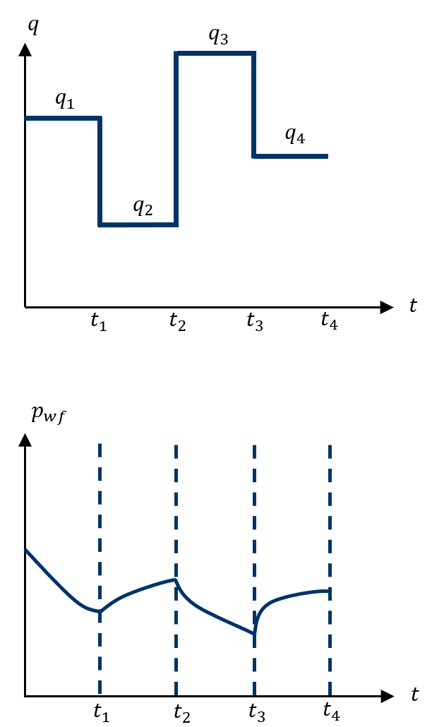
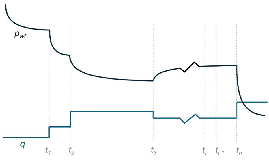
In practical well testing, production rates often vary over the course of a test due to operational constraints or intentional rate changes. Superposition in time is a mathematical technique that allows the pressure response for such variable-rate histories to be calculated by summing the effects of individual constant-rate segments. The concept is based on the linearity of the diffusivity equation under the assumptions of single-phase, slightly compressible flow in a homogeneous reservoir. Each rate change is treated as the start of a new constant-rate period, with its magnitude defined as the difference between the new rate and the previous rate. The total pressure response is obtained by adding contributions from each of these rate increments.

This approach is not limited to step-rate changes; it is also applied to approximately varying rates by decomposing them into a series of small constant-rate intervals. The technique ensures that data acquired under different rates can be combined on a common diagnostic plot—such as a semi-log or log–log plot—while preserving the underlying flow regime behavior. Superposition time functions, which adjust the time variable for each rate segment, are derived according to the specific flow regime being analyzed (e.g., radial, linear, or bilinear flow). By correctly applying superposition in time, variable-rate drawdown tests can be interpreted using the same analytical frameworks developed for constant-rate conditions, improving the reliability of permeability and skin estimates in real-world testing scenarios.

Consider a shut-in well that is subsequently produced in a sequence of constant-rate periods, each with a defined duration. To determine the total pressure drop at the sandface at a given time $t_4​$​, the response is calculated by summing the pressure changes generated during each constant-rate interval, applied in the order and timing of the rate history. This resultant pressure solution is obtained by superimposing the individual constant-rate analytical solutions corresponding to each step in the rate sequence.

$$\begin{equation} (\Delta p)_{\text{total}} = (\Delta p)_1 + (\Delta p)_2 + (\Delta p)_3 + (\Delta p)_4 \end{equation}$$

Where,

$$\begin{equation} (\Delta p)_1 = \left[\frac{162.6(q_1-0)B\mu}{kh}\right] \times \left[\log\left(\frac{kt_4}{\phi\mu c_t r_w^2}\right) - 3.23 + 0.87s\right] \end{equation}$$

$$\begin{equation} (\Delta p)_2 = \left[\frac{162.6(q_2-q_1)B\mu}{kh}\right] \times \left[\log\left(\frac{k(t_4-t_1)}{\phi\mu c_t r_w^2}\right) - 3.23 + 0.87s\right] \end{equation}$$

$$\begin{equation} (\Delta p)_3 = \left[\frac{162.6(q_3-q_2)B\mu}{kh}\right] \times \left[\log\left(\frac{k(t_4-t_2)}{\phi\mu c_t r_w^2}\right) - 3.23 + 0.87s\right] \end{equation}$$

$$\begin{equation} (\Delta p)_4 = \left[\frac{162.6(q_4-q_3)B\mu}{kh}\right] \times \left[\log\left(\frac{k(t_4-t_3)}{\phi\mu c_t r_w^2}\right) - 3.23 + 0.87s\right] \end{equation}$$

For a well that has undergone $n​$ discrete rate changes during its production history. The objective is to determine the wellbore pressure response for this variable-rate schedule. This is achieved by applying the principle of superposition in time as:

$$\begin{equation} \frac{p_i - p_{wf}}{q_n} = m'\sum_{j=1}^{n}\left[\frac{(q_j - q_{j-1})}{q_n}\log(t - t_{j-1})\right] + m'\left[\log\left(\frac{k}{\phi\mu c_t r_w^2}\right) - 3.23 + 0.869s\right] \end{equation}$$

$$\begin{equation*} \text{for } q_n \neq 0, \end{equation*}$$

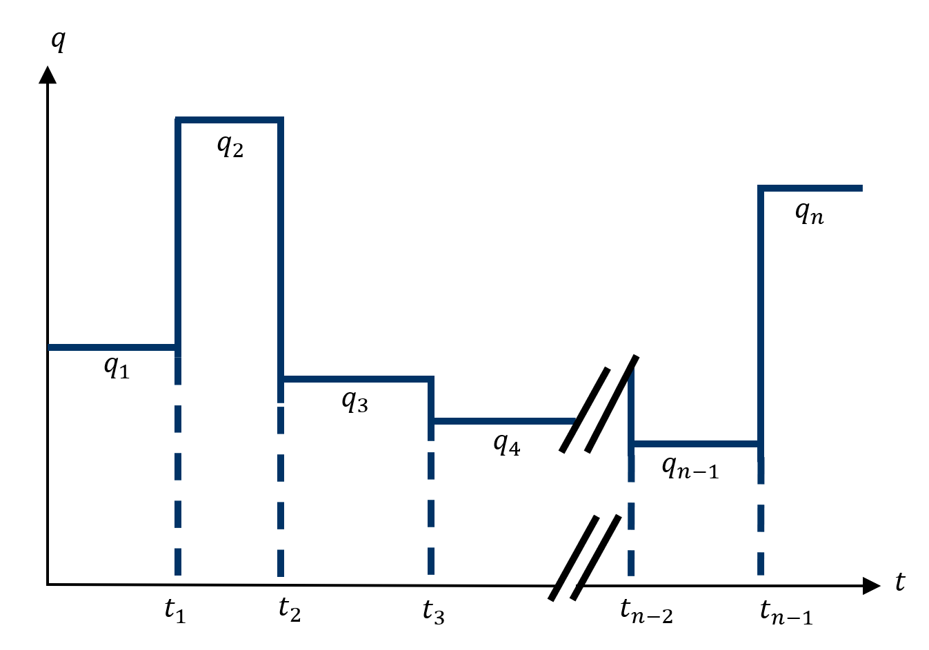
Where,

$$\begin{equation} m' = 162.6B\mu / kh \end{equation}$$

Buildup Test

Pressure buildup testing is one of the most widely used well testing techniques in the industry. A key advantage is that it does not require the same level of continuous operational supervision as some other testing methods. When the well is shut in during the transient period, a buildup test allows direct determination of $p_i​$​, the initial reservoir pressure at the measurement depth. If the shut-in period extends into the semi-steady state, the average reservoir pressure within the drainage area can also be estimated.

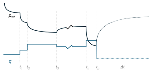
A pressure buildup test begins after the well has been flowing steadily at a constant rate $q​$ for a defined period $t_p​$. Once the well is shut in, the bottomhole pressure $p_{ws}​$ is recorded as it rises over time.

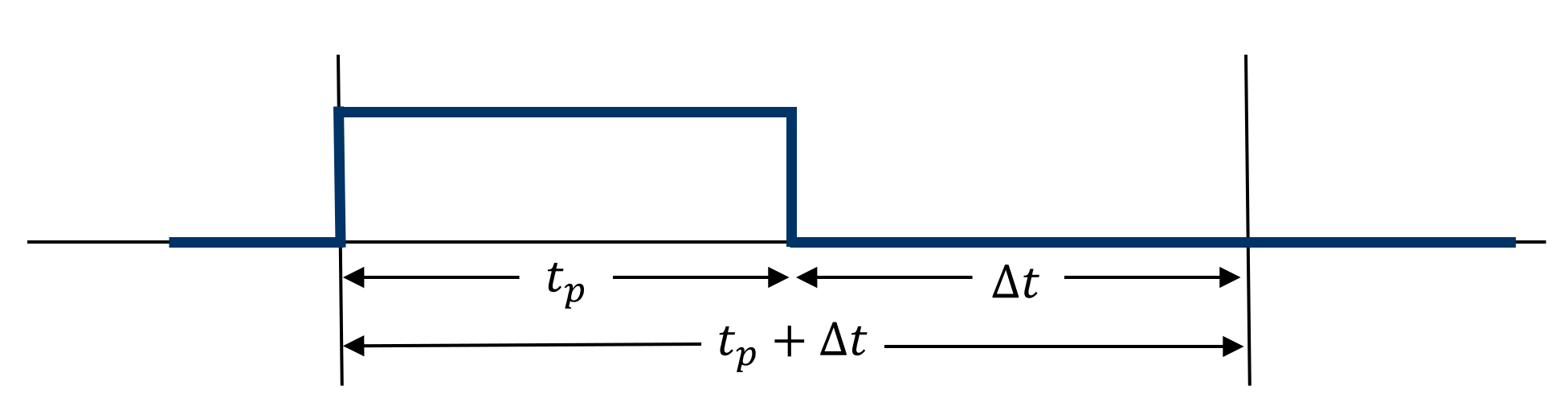
To represent this process mathematically, we can think of it as two separate rate events: the initial startup from zero to $q​$ at $t=0​$, and the subsequent drop from $q​$ to zero at $t = t_p​$ when the shut-in occurs. Because the diffusivity equation describing pressure propagation (Eq. 4) in porous media is linear, the pressure response during the buildup is obtained by superimposing the effects of these two rate changes. Analytical techniques such as the Horner plot or equivalent time methods like that of Agarwal (1980) can then be applied to interpret the resulting pressure data.

The pressure change resulting from production at a constant rate $q​$ at time $t=0​$ can be expressed as follows:

$$\begin{equation} \Delta p_{+q} = -\frac{162.6qB\mu}{kh}\left[\log t + \log\left(\frac{k}{\phi\mu c_t r_w^2}\right) - 3.23 + 0.869s\right] \end{equation}$$

The corresponding pressure change resulting from a rate decrease of “$-q​$” starting at time $t = t_p​$​ can be written as:

$$\begin{equation} \Delta p_{-q} = +\frac{162.6qB\mu}{kh}\left[\log(\Delta t) + \log\left(\frac{k}{\phi\mu c_t r_w^2}\right) - 3.23 + 0.869s\right] \end{equation}$$

Here, $Δt​$ is defined as $Δt=t−tp​$. The shut-in bottomhole pressure during the buildup period can then be determined using The Horner Method

Horner Method

Eqs. (28) and Eqs. (29) can be rearranged to obtain:

$$\begin{equation} p_{ws}(\Delta t) = p_i - \frac{162.6 q B \mu}{kh} \log\left(\frac{t_p + \Delta t}{\Delta t}\right) \end{equation}$$

By expressing Eq. 30 in the form $y=mx+b​$, it becomes clear that when buildup data under infinite-acting radial flow conditions are plotted as $p_{ws}(t)​$ versus $log[tp+Δt]/ Δt​$, the result should be a straight line. The slope of this line,

$$\begin{equation*} m = -\frac{162.6qB\mu}{kh} \end{equation*}$$

Where the intercept, $b = p_i​$ represents the initial reservoir pressure at the measurement depth.

The ratio $(tp+Δt)/Δt​$ is known as the Horner time ratio (HTR), and plotting pressure on a semi-log scale against the logarithm of HTR produces what is referred to as a Horner plot. As the shut-in period $(Δt)​$ increases, HTR decreases. Although the standard presentation uses increasing HTR from left to right, the plot may also be arranged so that time progresses in the conventional left-to-right direction.

Agarwal Equivalent-Time Method

In 1980, Agarwal proposed the concept of equivalent time as a means to interpret buildup tests using drawdown-type curves. This transformation allows pressure data from a buildup to be analyzed as though it were obtained during a continuous drawdown, thereby simplifying the use of existing type curves. Beyond buildup interpretation, Agarwal also demonstrated that the same concept can be adapted for semi-log straight-line analysis.

Mathematically, the flowing bottomhole pressure at the end of the production period, $p_{wf}​$ ​, can be expressed in terms of the equivalent time formulation as:

$$\begin{equation} p_{wf}(t_p) = p_i - \frac{162.6qB\mu}{kh}\left[\log(t_p) + \log\left(\frac{k}{\phi\mu c_t r_w^2}\right) - 3.23 + 0.869s\right] \end{equation}$$

Combining Eqs. * and **, we have

$$\begin{equation} p_{ws}(\Delta t) = p_{wf} + \frac{162.6qB\mu}{kh}\left[\log(\Delta t) + \log\left(\frac{k}{\phi\mu c_t r_w^2}\right) - 3.23 + 0.869s\right] \end{equation}$$

where $Δt_e​$​ represents the equivalent time, defined by:

$$\begin{equation} \Delta t_e = \frac{t_p \Delta t}{t_p + \Delta t} \end{equation}$$

Permeability and skin can be determined from the slope and intercept of a semi-log plot, similar to the Horner time plot.

Impact of Wellbore Storage on Early-Time Pressure Behavior

In classical well test theory, it is often assumed that a well can be opened for drawdown or closed for buildup instantaneously, with the change in flow rate immediately transmitted to the reservoir. Analytical models such as the infinite-acting radial flow formulation further idealize the process by assuming that the sandface rate rises instantly from zero to a constant value at the start of a drawdown, or falls immediately to zero at the onset of a buildup.

In reality, this assumption is rarely valid due to the finite volume and compressibility of fluid within the wellbore. When a well is opened at the surface, the initial production originates from the expansion of the wellbore fluid, not directly from the reservoir. As this stored fluid is produced, the sandface rate increases gradually, approaching the target production rate asymptotically. Conversely, when a well is shut in after flowing, reservoir fluid continues to enter the wellbore for a short time before the sandface rate declines to zero. This residual inflow during shut-in—commonly referred to as afterflow—is a key signature of wellbore storage.

If the well is equipped with downhole valves or a packer-tubing assembly, it is possible to reduce the volume of wellbore fluid exposed to compressibility effects, thereby minimizing wellbore storage. However, in most cases, the well is opened or closed at the surface, which amplifies early-time deviations from the idealized response.

Wellbore storage can significantly distort the early portion of a pressure transient record in both drawdown and buildup tests, often masking the reservoir’s true behavior. In situations of constant wellbore storage—such as single-phase flow or fixed liquid level wells—the storage coefficient remains constant, simplifying its analytical treatment. More complex conditions, such as multiphase flow or changing liquid levels, result in variable wellbore storage, which is more challenging to model accurately. Recognizing and correctly accounting for wellbore storage effects are critical to reliable estimation of key reservoir parameters, particularly permeability and skin factor.

Graph Scales in Well Test Interpretation

Graph scales are a fundamental aspect of well test interpretation because they influence how data trends are visualized and how flow regimes are recognized. The three most commonly used scales are Cartesian, semi-log, and log-log, each offering different benefits for highlighting specific flow periods and diagnosing reservoir behavior.

On a Cartesian scale, both axes are linear. This scale preserves the true magnitude of changes over time and is particularly useful for visualizing the overall trend of a dataset. However, for pressure transient data that spans several orders of magnitude in time, a Cartesian plot compresses early-time data and stretches late-time data, which can obscure important early-time behaviors. For instance, in a typical test, 90% of the data points may occupy 90% of the time axis, leaving the first 10% of the time—where wellbore storage and near-wellbore effects occur—highly compressed and difficult to analyze.

Logarithmic scales address this by compressing long time periods and expanding short ones. On a logarithmic scale, one log cycle corresponds to a tenfold change in value. This property allows both early and late-time data to be displayed in a balanced way, making it easier to observe transient flow regimes. semi-log plots (linear pressure axis, logarithmic time axis) are particularly suited for identifying radial flow, where the pressure change versus log time yields a straight-line segment. Log-log plots (logarithmic pressure change and derivative versus logarithmic time) are widely used for diagnostic purposes, as they preserve curve shape under proportional scaling of both axes and are the basis for type-curve matching.

An important feature of log scales is proportional spacing: points with the same multiplicative ratio (e.g., 2 to 6, 6 to 18, 18 to 54) appear evenly spaced on the axis, regardless of their absolute value. This invariance allows different datasets or models to be directly compared by shifting curves horizontally or vertically without altering their shape.

The choice of scale, however, can hide as much as it reveals. Damage effects, boundary signals, or derivative anomalies may be invisible on one scale yet clearly identifiable on another. For example, a dataset may appear to match a model perfectly on a Cartesian plot, but the mismatch becomes obvious when plotted on a semi-log scale. Similarly, subtle flow regime changes seen in a log-log derivative plot may be lost entirely in a Cartesian or semi-log view.

Because each scale emphasizes different aspects of the data while de-emphasizing others, best practice in well test interpretation is to examine the dataset on multiple scales. This ensures that no significant feature is overlooked, whether it occurs in the early, middle, or late stages of the test.

Practical Notes on Plotting Scales

• In a Cartesian time plot, late-time data occupies most of the horizontal axis, causing early-time behavior to appear condensed.

• In a logarithmic time plot, the time axis is divided into log cycles, each containing a similar proportion of the data points, making early and late-time periods easier to compare.

• For transient well tests, the final log cycle on a logarithmic time scale typically contains the majority of the data points recorded during the test.

• On a logarithmic axis, values that change by the same multiplicative factor are equally spaced, regardless of their magnitude.

• A semi-log format (linear pressure, logarithmic time) stretches the early-time region, making straight-line trends associated with radial flow easier to detect.

• A log-log format (logarithmic pressure change and derivative, logarithmic time) maintains curve shapes under proportional scaling of both axes, which is important for diagnostic plots and type-curve matching.

• Evaluating data on more than one scale reduces the risk of overlooking important features, as each scale emphasizes different parts of the dataset.