whitson+ - Well Test Certification
1. Introduction
Complete the steps outlined below to become a Well Test certified whitson+ user. It includes performing three analyses: a chow pressure group (CPG) test, a diagnostic fracture injection test (DFIT) and Devon Quantification of Interference (DQI). You can learn more about the respective tests in the manual where we cover most of the theoretical fundamentals:
- CPG - Chow Pressure Group Test
- DFIT - Diagnostic Fracture Injection Test
- DQI - Devon Quantification of Interference
Those certified have the software skills necessary to complete most CPG and DFIT evaluation projects in tight unconventionals.
Need help?
Send an e-mail to support@whitson.com.
1.1. Before Starting
Make sure you have watched these three videos in the Getting Started part of the manual (click here).
- Login (1 min)
- Overview of important basics (3 min 30 sec)
- Zoom Plots (3 min)
1.2. Create a Project
- Go to the Projects module in the navigation panel.
- Click ADD PROJECT up to the right.
- Name the project "your name - whitson certificate".
- Click SAVE.
- All steps are shown in the .gif above.
1.3. Upload Required Data
You can download the files required for each test individually and upload using the mass upload dialog box on the wells page, as shown in the sections below.
Alternatively, all the data required for this exercise has been bundled into a mass upload file, ready to be uploaded, in the Mass Upload -> Examples section.
- Click MASS UPLOAD up to the right.
- In the pop-up window, select EXAMPLES
- Search for Well Test Examples - DFIT/CPG/DQI and click UPLOAD
- All the data will be uploaded into the project. You can then close the Mass Upload pop-up window.
- All steps are shown in the .gif above.
2. CPG Workflow
2.1. Before Getting Started
2.1.1. Recommended Data Size for CPG Tests
CPG datasets could be far higher frequency than needed. Datasets can vary from second by second frequency to tens of seconds for the entirety of the test. This can be harder to handle, and make the numerical derivative calculation unwieldy.
Rather than uploading high-resolution data, we recommend resampling the dataset externally using pressure increments of 5 to 10 psi. This reduces file size and improves performance. For best results, keep the number of uploaded data rows between 30,000 and 40,000. To learn how to resample your data within whitson+, see the resampling section here.
2.1.2. Data Truncation
The Truncate Data feature in the Well Test modules (CPG and DQI) allows users to remove unwanted portions of the dataset and focus the analysis on a specific time range. This is useful for excluding early-time noise, late-time operational changes, or any data outside the period of interest.
Truncation Methods
-
Date-Based Truncation
Users can manually define the truncation window by selecting a truncate start date and truncate end date using the calendar controls. All data outside the selected range is removed.
-
Visual Truncation
Users can visually select the data range to retain directly on the plot. A black dotted line marks the start of the retained data, and a blue dotted line marks the end. Data before the black line and after the blue line will be deleted.
Data size
For these certificate steps, there is no need to worry about data size.
2.2. Chow Pressure Group Analysis
You can analyze the Chow Pressure Group for the monitoring well by navigating to the Chow Pressure Group feature under Well Testing.
2.2.1.Pressure Difference plot
- Go to the Chow Pressure Group section in the Well Testing module in the navigation panel.
- On the Pressure Difference plot on the top-left move the CPG fit line (yellow, dashed line) to match the pressure difference data prior to the well put-on-production (POP) date.
- You can adjust the slope by:
- Manually moving the fit line on the plot (grab the line at the ends to adjust),
- Changing the Constant and Exponent of the power-law fit line directly in the input, or
- Lasso fit the pressure data prior to POP using the lasso tool to auto-adjust the fit line.
- Adjust the gray, dashed vertical line along the monitoring well data to the date and time when offset production well is POP.
- The difference in these CPG fit and the data is plotted along with it's derivative as \(\Delta p, \Delta p'\) vs. time plot (bottom-right). Observe the changes in this plot as the fit line is changed.
- All steps are shown in the .gif above.
2.2.2. \(\Delta p, \Delta p'\) vs. Time Plot
On the \(\Delta p, \Delta p'\) vs. time plot (bottom-right), you can switch between the derivative calculation techniques mentioned above - by selecting from the dropdown list for 'Derivative Function'.
Notice how switching between the different methods and window sizes in the GIF above changes the derivative shape and hence, impacts the CPG values calculated.
Note
Bourdet Derivative and Weighted Central Difference give you the additional option to modify the smoothing window as a log cycle fraction or a step size respectively. Both these methods are higher in accuracy compared to simply using the Central Difference with a fixed step size.
2.2.3. Plot Integral Function
Use the integral icon Plot Integral icon in the plot options to recalculate the pressure as an integral and recompute the derivative based on the derivative function selected above. You can also use the LOWESS Filter toggle with an appropriate smoothing window in log cycles to smooth noisy pressure data.
These methods inherently smooths the pressure response, and removes additional noise that may be a part of the dataset to create a much smoother derivative and CPG plot. Since the pressure integral is already smooth, a smaller window size can be used for derivative calculation.
2.2.4. CPG Value
Lastly, on the Chow Pressure Group plot, you can set the final CPG value in three ways:
- Move the horizontal dashed line to track the average of the CPG values after POP date.
- You can also adjust it by entering a value for CPG fit.
- You can also select the CPG based on the slope in \(\Delta p\).
This is the CPG value that indicates the level of interference between the production well and the monitoring well.
3. DFIT Workflow
3.1. Before Getting Started
3.1.1. Recommended Data Size for DFIT Tests
DFIT datasets could be far higher frequency than needed. Datasets can vary from second by second frequency to tens of seconds for the entirety of the test. This can be harder to handle, and make the numerical derivative calculation unweildy.
Instead of uploading such high resolution data, the recommended practice is to smooth the dataset externally by resampling the data in terms of pressure increments of 5 to 10 psi. Note that there is a further reduction using pressure increments of 30 psi in the DFIT feature to improve speed for dynamic calculations too. However, it is good practice to limit the number of data rows uploaded into whitson+ to between 30,000 and 40,000. To learn how to resample your data within whitson+, see the resampling section here.
Data size
For these certificate steps, there is no need to worry about data size.
3.1.2. Choices/Assumptions That Need to be Made:
- Choose the preclosure method of choice (G-function and H-function with Radial and PKN fractures) - recommended to go with H-function method with radial fracture geometry.
- Choose the postclosure method of choice based on late time impulse flow signatures (linear/radial flow). Note that the preclosure assumption on fracture geometry also auto-applies to the post closure analysis.
Some notes on automated selections in the software
These preliminary steps are done automatically, you may still need to review these selections
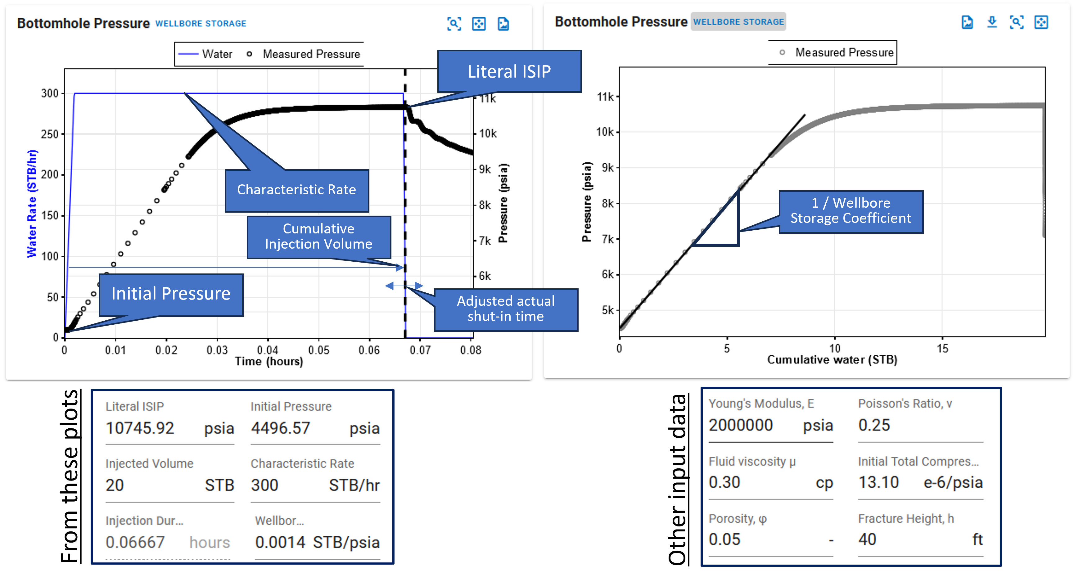
- Shut in is detected automatically from zero rate. Instantaneous ISIP is identified as the pressure right after the well is shut in.
- Initial pressure, Pw,init is chosen as the first point in the pressure data.
- Cumulative injection volume, and maximum sustained injection rate until the shut in time (characteristic rate), is calculated from the plot. Injection duration is autocomputed from the two above.
- Slope in the pressure vs cumulative injection (Wellbore Storage plot) is detected to calculate the wellbore storage. If rate data is unavailable, just enter the values cumulative injected volume, maximum sustained rate, and wellbore storage.
- Pore pressure is calculated automatically by extrapolating the post closure linear transient (default) on the inverse square root time plot.
3.2. Parameters
- Go to the DFIT section in the Well Testing module in the navigation panel.
- Review the automatic selection of parameters from the plots, i.e. Literal ISIP, initial pressure, injected volume, characteristic rate, wellbore storage coefficient, minimum .
- Enter the additional parameters relevant for the calculation, i.e. Young's modulus, Poisson's ratio, reservoir fluid viscosity and compressibility.
3.3. Physical Assumptions
Dropdowns for preclosure method and post closure methods allow you to switch between the different methods as well as fracture geometry assumption.
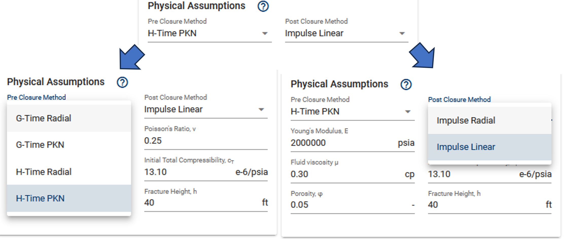
- Selection of frac geometry (Radial/PKN) in preclosure methods enforces the same geometry assumption in postclosure methods.
Note that PKN fractures will need fracture height as an additional input.
3.4. G-Function Plot
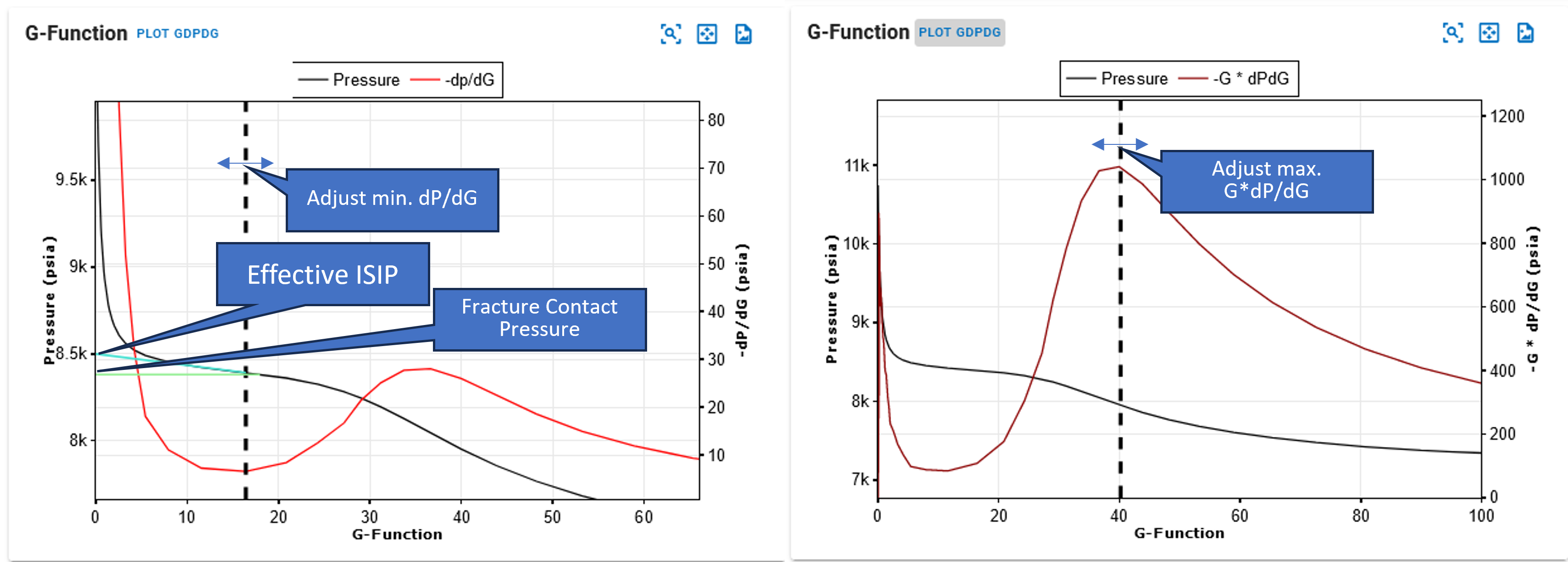
- Identify point of minimum in the G-Function plot.
- Identify point of maximum.
- All steps are shown in the .gif above.
This automatically computes the effective ISIP, Fracture Contact Pressure and Minimum Principal Stress and are used in subsequent calculations for permeability. The resolved values could be overwritten.
3.5. Late Time Shut-In Identification
- Click the slash icon to the top right in the dp after shut-in plot to add a slope.
- Identify if the late time shut in data has post closure transients
- Linear flow will have a half-slope signature and radial flow (rare, beware of false radial signatures in gas wells) will have a unit slope signature.
- Add the interpretation lines if needed and switch the plot (to the right) to impulse radial flow plot by clicking the 'plot radial' button.
- Align the slope to the pressure points near x=0 and let that extrapolate to calculate the pore pressure.
- All steps are shown in the .gif above.
3.6. Permeability Computation
Calculation should dynamically run when any of the inputs are changed to compute permeability. If you have reliable post closure transients, use the permeability estimates from the postclosure analysis. Correct preclosure permeability estimates by about 1.5 since they statistically tend to overestimate the permeability.
4. DQI Workflow
4.1. Before Getting Started
4.1.1. Recommended Data Size for DQI Tests
DQI datasets could be far higher frequency than needed. Datasets can vary from second by second frequency to tens of seconds for the entirety of the test. This can be harder to handle, and make the numerical derivative calculation unweildy.
Rather than uploading high-resolution data, we recommend resampling the dataset externally using pressure increments of 5 to 10 psi. This reduces file size and improves performance. For best results, keep the number of uploaded data rows between 30,000 and 40,000. To learn how to resample your data within whitson+, see the resampling section here.
4.1.2. Data Truncation
The Truncate Data feature in the Well Test modules (CPG and DQI) allows users to remove unwanted portions of the dataset and focus the analysis on a specific time range. This is useful for excluding early-time noise, late-time operational changes, or any data outside the period of interest.
Truncation Methods
-
Date-Based Truncation
Users can manually define the truncation window by selecting a truncate start date and truncate end date using the calendar controls. All data outside the selected range is removed.
-
Visual Truncation
Users can visually select the data range to retain directly on the plot. A black dotted line marks the start of the retained data, and a blue dotted line marks the end. Data before the black line and after the blue line will be deleted.
Data size
For these certificate steps, there is no need to worry about data size.
4.2. PVT
You need PVT initialization to gather fluid properties like fluid compressibility, viscosity, etc. from the black oil tables. You want to ensure that the PVT initialization matches the fluid that can be expected between these wells.
- Go to the Scenarios module in the navigation panel.
- Initialize PVT with 100% water saturation
- Go to the PVT module in the navigation panel.
- Open the Reservoir Fluid Composition Input Card
- Click SAVE.
- All steps are shown in the .gif above.
For a DQI test shortly after the initial stimulation in the offset well prior to the well being produced, initialize PVT with 100% water saturation - this is what we'll do here in this example dataset, as shown in the GIF above.
For tests where the well pair has been producing hydrocarbons, initialize the PVT with the GOR associated with the reservoir fluid in place.
4.3. Align the POP Line of the Offset Well
- Go to the Production Data module in the navigation panel.
- Taking a quick look at the pressures in the production data.
- Go to the DQI section in the Well Testing module in the navigation panel.
- Set the offset well POP to 1.48 days.
- All steps are shown in the .gif above.
You can enter it in or move the vertical dashed line graphically to the point in time when the offset well is POP'ed.
4.4. Align the Line to Pressure Trend Before POP
- Fit the prior pressure trend by moving and adjusting the slope line to align with the stabilized pressure trend prior to POP.
- You can do this manually or you can just lasso fit the stabilized pressure data.
- All steps are shown in the .gif above.
Notice how the pressure and pressure derivative vs time after POP plot is dynamically recalculated as you make adjustments to the prior pressure trend.
4.5. Autofit
Once the prior pressure trend and POP is picked, we have a plot of.
- Click the AUTOFIT button (off to the top-left of the page)
-
This fits the analytical model to the pressure and pressure derivative data to determine model parameters:
- α (controls hydraulic diffusivity) - impacts the timing of the onset of pressure interference.
- κ (controls fracture conductivity) - impacts the shape of the curve after the interference. Resolving these two parameters allows you to calculate the fracture conductivity 'κ' and maximum possible drainage length along the fracture, 'L', given W (fracture width or aperture) and (change in fracture aperture with change in pressure) and other parameters.
Assessing fit quality
The priority is to ensure that the fit matches the initial response - the first 10s or 100s of psi. The analytical solution is not expected to match the transient after the initial response.
-
Then the Ld is calculated, given the well spacing, 'y'.
- This is plotted in the empirical correlation developed to calculate DPI, given the .
- The resulting DPI should be close to 95%.
- All steps are shown in the .gif above.
Note down the α and κ, both of which are indicators of good or bad well-pair connectivity, apart from the DPI. This will help you rank the well-pair connectivity on large scale tests with multiple well pairs.
Do It Yourself
Did you know that the CPG and DQI datasets are both interference tests between different well pairs? This means that the CPG dataset can be used to calculate the DPI for that well pair and the DQI dataset can be used to calculate the CPG value for the other well pair.
Do you want to give this a try? Use the wells in your project and assess the interference datasets with an alternate techniques.
Report the answers in your submission below for some extra kudos!
Want to Learn More?
Schedule a Well Test session with one of our engineers. Contact support@whitson.com.
Done?
When you are done analyzing your Well Tests please:
- Send an e-mail to certification@whitson.com
- Make the subject: "whitson+ Well Test certificate: [YOUR NAME HERE]".
- Include the link to your project.
- If you have any notes, comments, or observations related to the well, feel free to share them with us. Also feedback on the user friendliness of the software is always appreciated.
After that we'll provide some feedback on your evaluation and issue your whitson+ certificate if all looks good.