whitson⁺ - PNR DCA Certification

1. Introduction

Complete the steps outlined below to become a PNR DCA certified whitson⁺ user. It includes performing workflow for two wells —one oil and one gas— with actual production data from the SPE Data Repository . Those certified have the software skills necessary to complete most PNR DCA projects in tight unconventionals.

Need help?

Send an e-mail to support@whitson.com.

1.1. Before Starting

Make sure you have watched these three videos in the Getting Started part of the manual (click here).

• Login (1 min)
• Overview of important basics (3 min 30 sec)
• Zoom Plots (3 min)

1.2. Create a Project

1. Go to the Projects module in the navigation panel.
2. Click ADD PROJECT up to the right.
3. Name the project "Your Name - whitson Certificate - PNR DCA".
4. Click SAVE.
5. All steps are shown in the .gif above.

1.3. Upload the Well Data

1. Click MASS UPLOAD up to the right.
2. In the pop-up window, select EXAMPLES
3. Search for PNR DCA Certificate Wells and click UPLOAD
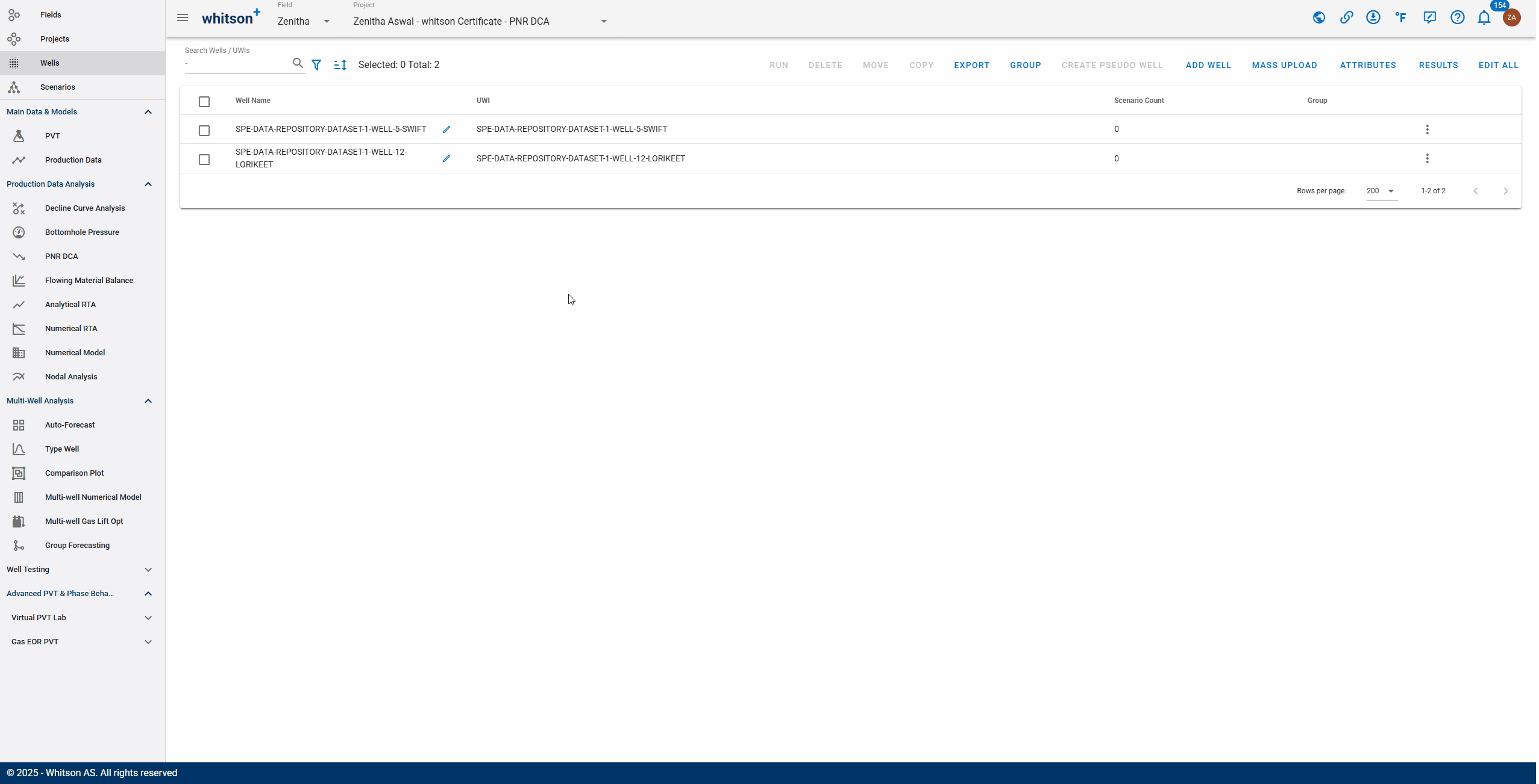
4. All the data will be uploaded into the project. You can then close the Mass Upload pop-up window.
5. All steps are shown in the GIF above.

2. Oil Well : SPE-DATA-REPOSITORY-DATASET-1-WELL-9-JAY

2.1. PVT

1. Click on the well named "SPE-DATA-REPOSITORY-DATASET-1-WELL-9-JAY"
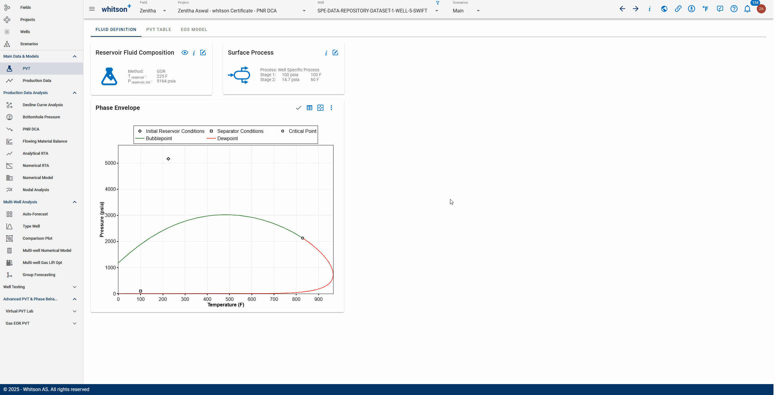
2. Go to the PVT module in the navigation panel.
3. Open the Reservoir Fluid Composition Input Card
4. Click SAVE.

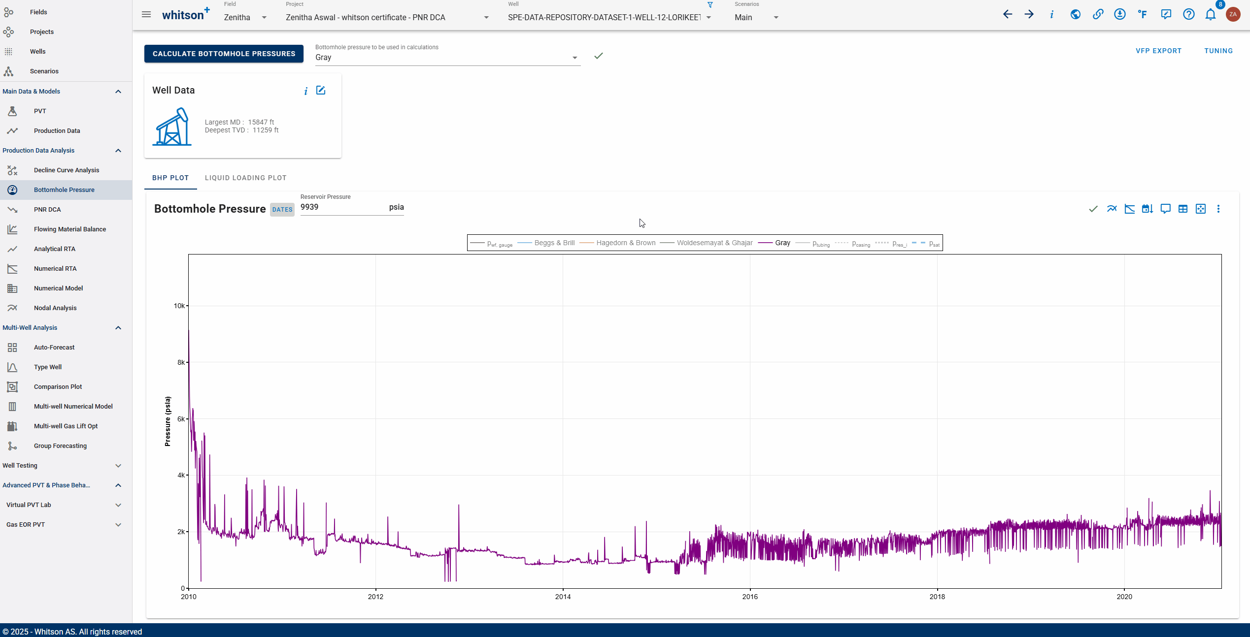
2.2. Bottomhole Pressure Calculations

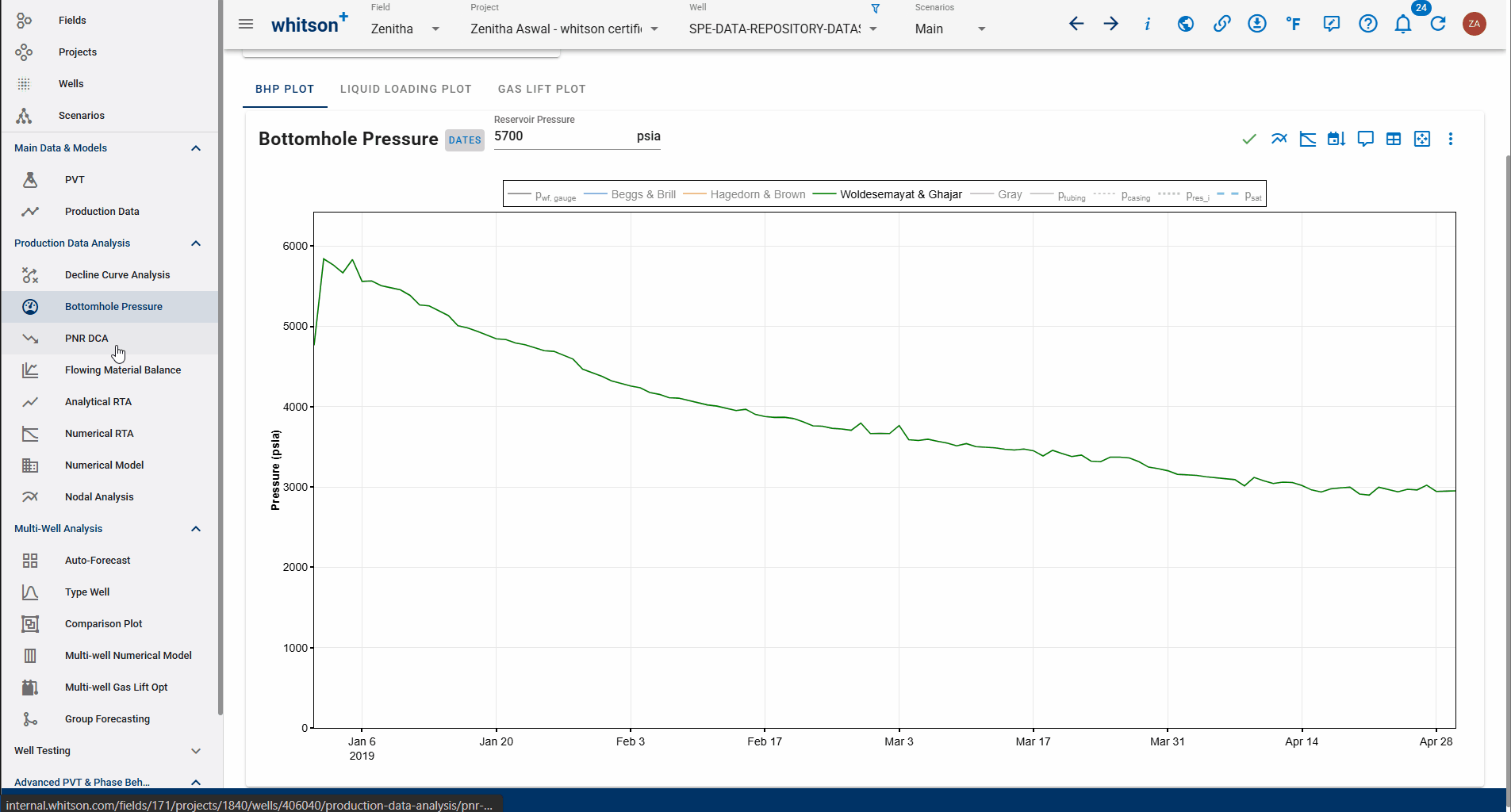
1. Go to the Bottomhole Pressure module in the navigation panel.
2. Click the CALCULATE BOTTOMHOLE PRESSURES button.
   • This will run the calculation for four different BHP correlations at the same time.
3. Select Woldesemayat and Ghajar as the "Bottomhole pressure to be used in calculations".
   • The dropdown menu can be found right of the CALCULATE BOTTOMHOLE PRESSURES button.
   • The selected BHP is used everywhere in the software where BHPs are required (FMB, PNR DCA, RTA, Numerical Model, Nodal Analysis).
4. To isolate the Woldesemayat and Ghajar calculation in the plot, double-click the legend.
5. All steps are shown in the .gif above.

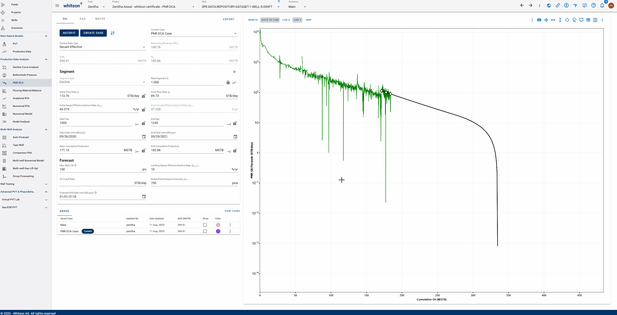
2.3. PNR DCA

2.3.1. Creating a PNR DCA Case

1. Click the CREATE CASE option and then select the Create Case For Oil to save the case.
2. Save the case as PNR DCA Case
3. All the steps are shown in the gif above.

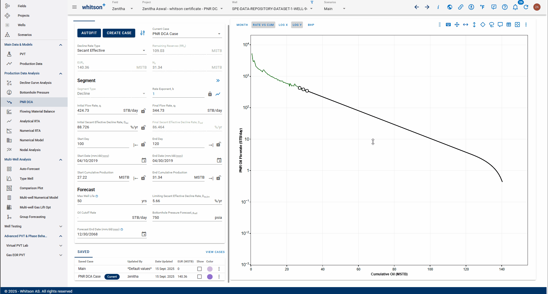
2.3.2. Manually Fitting the Segment

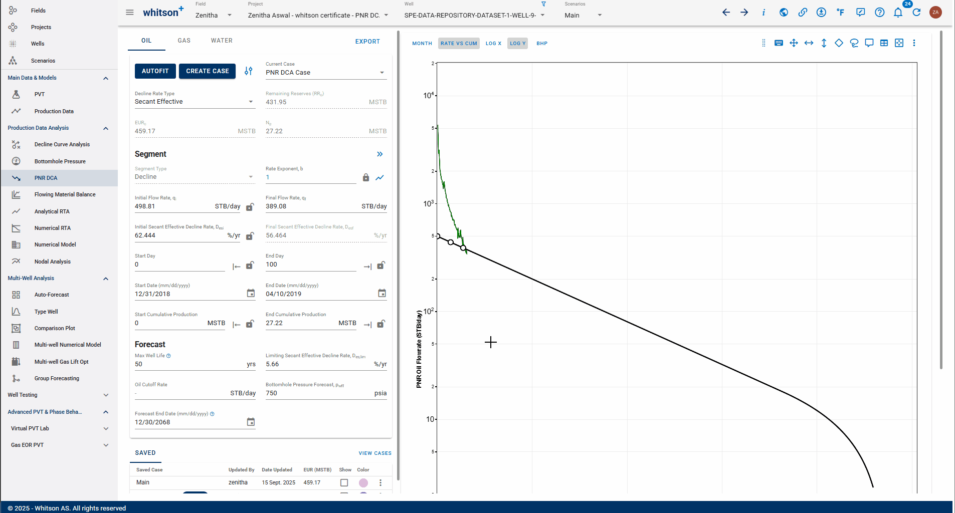
1. Go to the PNR DCA module.
2. Keep the Rate Exponent (b-value) at its default of 1.0.
3. Click the arrow icon next to End Day and set it to the last available historical production day (~120 days).
4. Set the Start Day to 100 days.
5. Use the Adjust Curve tool (vertical double-arrow ↕ icon in the top-right corner of the plot, as shown in the GIF above) to align the decline curve with the historical oil data. If additional alignment is needed, use the Shift Curve tool (horizontal double-arrow or four-way arrow icon) to move the entire curve and improve the match with the historical data.
   • The curve should approximately match an initial rate of 425 STB/day and a final rate of 345 STB/day.

Shifting or adjusting the segment

There are three options to shift or adjust the segments points without changing the rate exponent.

• Shift entire decline
• Shift segment points along the decline curve
• Adjust shape of decline curve

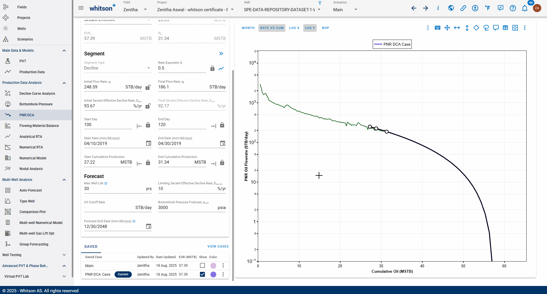
2.3.3. Adjusting Forecast Parameter

1. To see the limiting decline start point, select Show limiting decline start point icon (as shown in the GIF above).
2. To view the BHP profile on the plot, enable the BHP option at the top left of the plot (as shown in the GIF above).
3. Set Max Well Life as 30 years.
4. Increase the Limiting Secant Effective Decline Rate, \(d_{sec}\) to 10%/yr
5. Increase the Bottomhole Pressure Forecast, \(P_{wff}\) to 3000 psia.
6. Adjust the fit manually using the Shifting or adjusting the segment tool as shown in the GIF above.

Bonus Question

Why Bottomhole Pressure Forecast, \(P_{wff}\) is set to 3000 psia?
Hint: Take into account the flowing BHP values between 100 and 120 days, and note that this case will be exported to the DCA module in the next section.

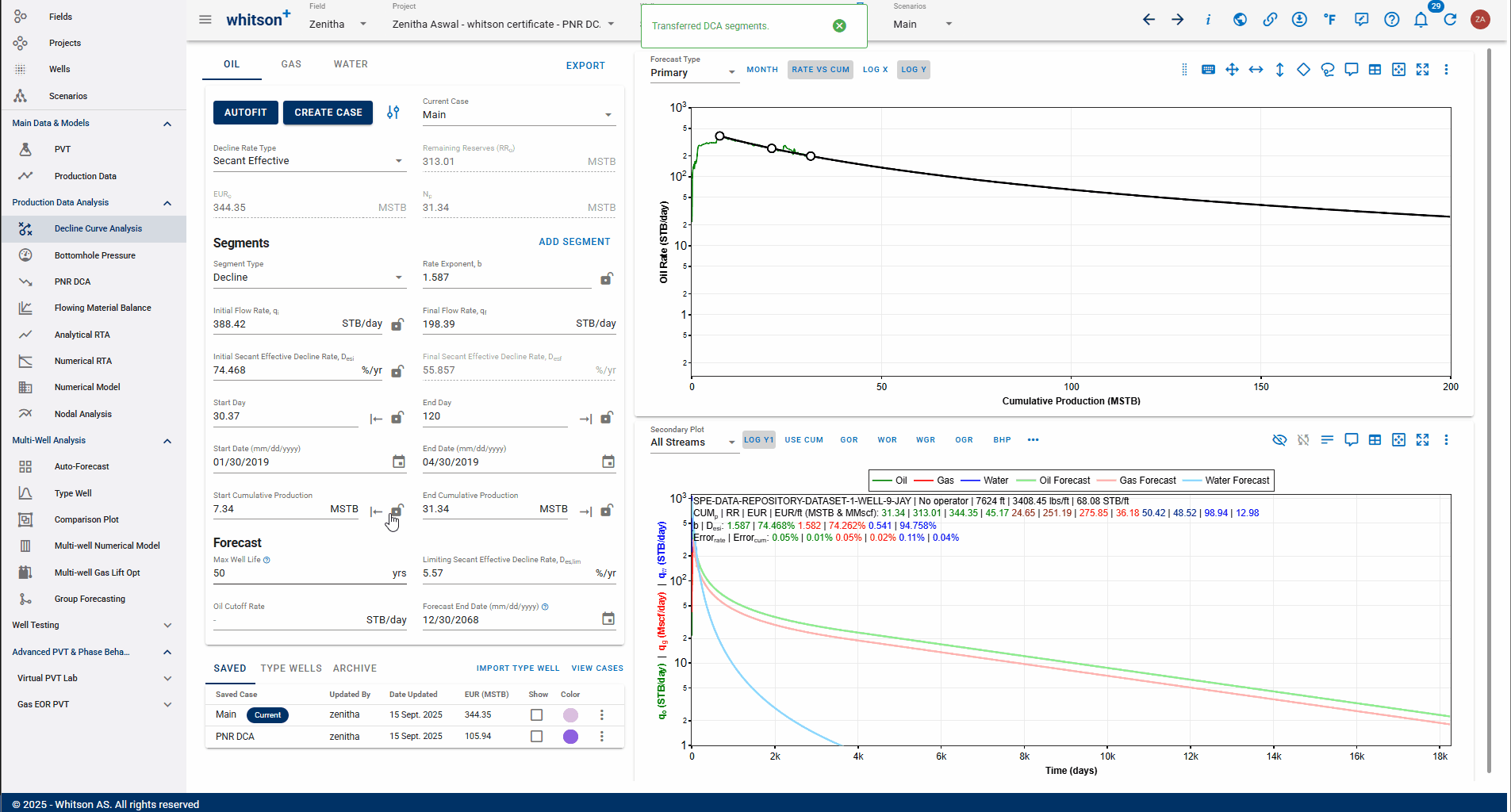
2.3.4. Exporting the segments to the DCA

1. Click the Export Segment Parameters icon (double arrows). This will export the current case (PNR DCA Case in this example).
2. Select the option Use Parameters in DCA Module.
3. Keep the default case name (PNR DCA) or rename it as desired.
4. Click SAVE. You will automatically be redirected to the DCA Module.

Exporting PNR DCA Segments to the DCA Module

When exporting PNR DCA segments to the DCA module, the PNR flow rate decline trend converges to the actual rate decline trend when bottomhole pressure is relatively stable and the pressure at abandonment is close to the flowing bottomhole pressure. This is because PNR flow rates are scaled by \((p_i − p_{wf,min})\), and when BHP is constant, the PNR fit align more closely with the DCA fit.

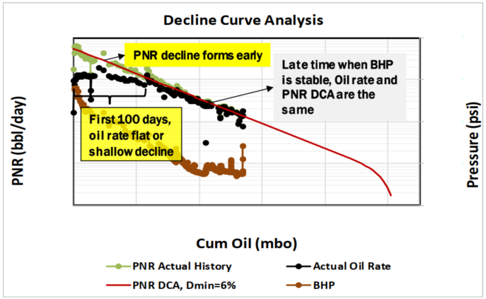
Source: Xie, Xueying (2025)

2.3.5. Comparing PNR DCA and DCA Forecast

1. In the DCA Module, let us change the Forecast parameters to be the same as the PNR DCA case.
   • Change the Max Well Life to 30 years
   • Increase the Limiting Secant Effective Decline Rate, \(d_{sec}\) to 10%/yr
2. Under the SAVED section, check the box for the PNR DCA Case to display its forecast on the plot.
3. Change the plot from RATE VS CUM to RATE VS TIME by disabling the RATE VS CUM option from the top left of the plot.
4. By default, the current case in the DCA Module is the DCA Main Case. First, note the EUR value for the default case. Then, switch the current case to the PNR DCA Case and observe the updated EUR value.
5. Check the box for the Main case under the SAVED section to display the DCA forecast on the plot. View the RATE VS TIME plot by disabling the RATE VS CUM option from the top left of the plot.

3. Gas well : SPE-DATA-REPOSITORY-DATASET-1-WELL-20-LOON

3.1. PVT

1. Go to the Wells module in the navigation module
2. Click on the well named "SPE-DATA-REPOSITORY-DATASET-1-WELL-20-LOON"
3. Go to the PVT module in the navigation panel.
4. Open the Reservoir Fluid Composition Input Card
5. Click SAVE.

3.2. Bottomhole Pressure Calculations

1. Go to the Bottomhole Pressure module in the navigation panel.
2. Click the CALCULATE BOTTOMHOLE PRESSURES button.
3. Select Gray as the "Bottomhole pressure to be used in calculations".
4. To isolate the Gray calculation in the plot, double-click the legend.
5. All steps are shown in the GIF above.

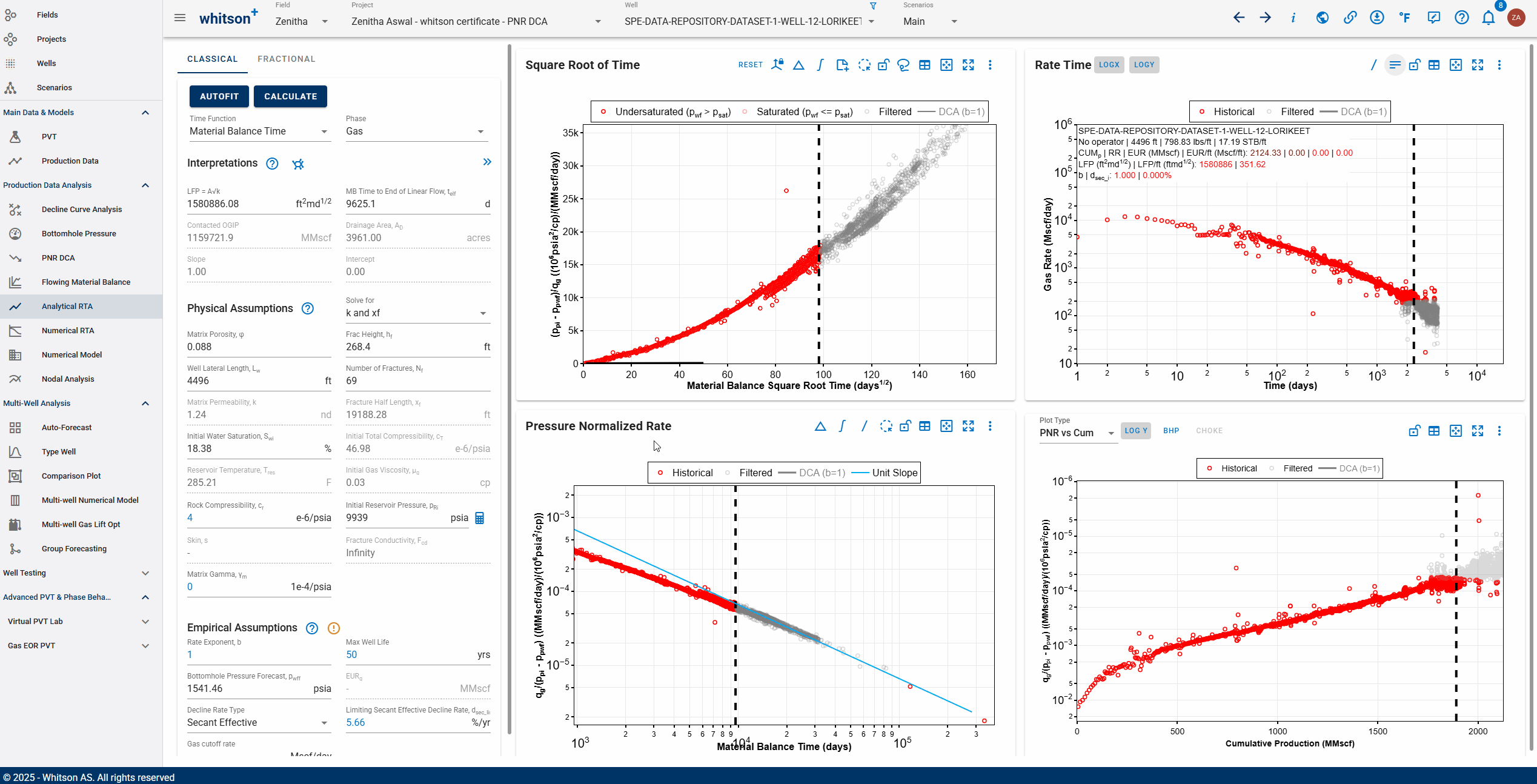
3.3. Analytical RTA

3.3.1. Identifying the Time to the End of Characteristic Flow

1. Go to the Analytical RTA module in the navigation panel.
2. In the Pressure Normalized Rate plot (bottom left), add a unit slope line (as shown in the GIF) and align it with the latest portion of the production history. The unit slope indicates the onset of the boundary-dominated flow regime.
3. Use the Lasso tool to highlight the Boundary Dominated Flow (BDF) region.
4. From the Rate Time plot (top right), BDF starts at around ~380 days (real time).

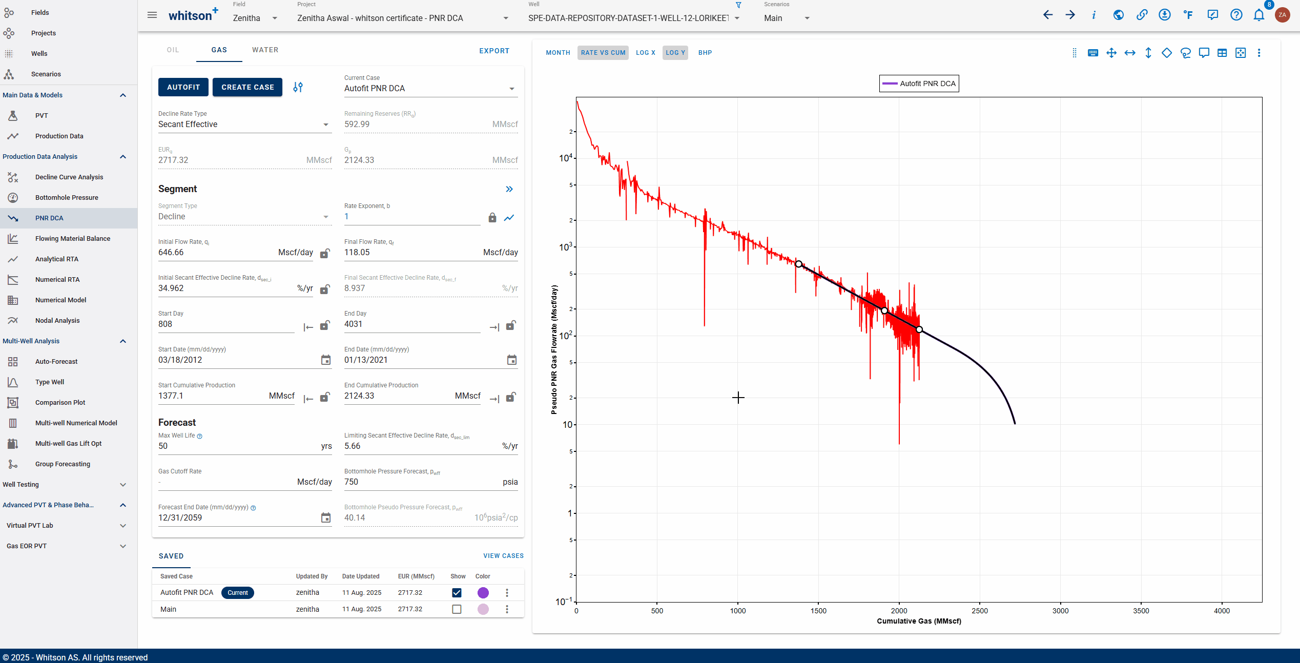
3.4. PNR DCA

3.4.1. Autofit

1. Go to the PNR DCA module in the navigation panel.
2. Click the CREATE CASE option and then select the Create Case For Gas to create a new autifit case.
3. Enter a case name, e.g., Autofit PNR DCA. The case will be created and can be seen under the SAVED Case section at the bottom.
4. Click Edit Autofit Setting to open the dialog box. Review the ranges for Peak Production Rate Ratio, Initial Nominal Decline Rate, Rate Exponent (b), and Noise Reduction. Leave the default values unchanged.
5. Click AUTOFIT to run the fit.

3.4.2. Fit Using Fractional RTA

1. Let us first create a new case by clicking the CREATE CASE option, then select Create Case for Gas.
2. Enter the case name FRTA PNR DCA. The newly created case will appear in the Saved section at the bottom.
3. Now, click the icon next to the Rate Exponent (b) field to open the Fractional RTA plot.
4. In the Fractional RTA window, set the Segment Start Day to 380 days (this corresponds to the time to start of boundary dominated flow found using the Analytical RTA module).
5. Fit the slope line to the data after 380 days to determine the rate exponent (around 0.6).
6. Click SAVE
7. All the steps are shown in the GIF above.

Is your fit not the same as us?

If your values or the fit is not the same as the above analysis, it is okay. It is not you, it is us. Our engineers are working to estimate the Di in the best possible manner. So for the time being you can manually put the Di value as 82.258 %/yr to get the best PNR DCA fit.

3.5. Want to Learn More?

Schedule a PNR DCA session with one of our engineers. Contact support@whitson.com.

4. Done?

When you are done with your PNR DCA please:

1. Send an e-mail to certification@whitson.com
2. Make the subject: "whitson⁺ PNR DCA certificate: [YOUR NAME HERE]".
3. Include the link to your project.
4. Report the following from your DCA and PNR DCA Module.
   1. EUR from the DCA and PNR DCA case for the oil well.
   2. EUR from the Autofit PNR DCA case for gas well.
   3. EUR from the FRTA PNR DCA case for gas well.
5. If you have any notes, comments, or observations related to the well, feel free to share them with us. Also feedback on the user friendliness of the software is always appreciated.

After that we'll provide some feedback on your evaluation and issue your whitson⁺ certificate if all looks good.

5. Want to Learn More?

Read more about the PNR DCA here: Pressure Normalized Rate (PNR) DCA