whitson+ - Nodal Analysis Certification
1. Introduction
Complete the steps outlined below to become a certified whitson+ user. It includes performing a nodal analysis workflow for two wells with actual production data from the SPE Data Repository . Those certified have the software skills necessary to complete most nodal analysis and completion evaluation projects in tight unconventionals.
We'll go over two kinds of analyses, typically performed via single point in time estimates from nodal analysis -
- Running completion design sensitivity tests to prevent a Marcellus dry gas well from liquid loading.
- Optimizing lift gas injection rate and gas lift design to maximize produced oil rate.
Need help?
Send an e-mail to support@whitson.com.
1.1. Before Starting
Make sure you have watched these three videos in the Getting Started part of the manual (click here).
- Login (1 min)
- Overview of important basics (3 min 30 sec)
- Zoom Plots (3 min)
1.2. Create a Project
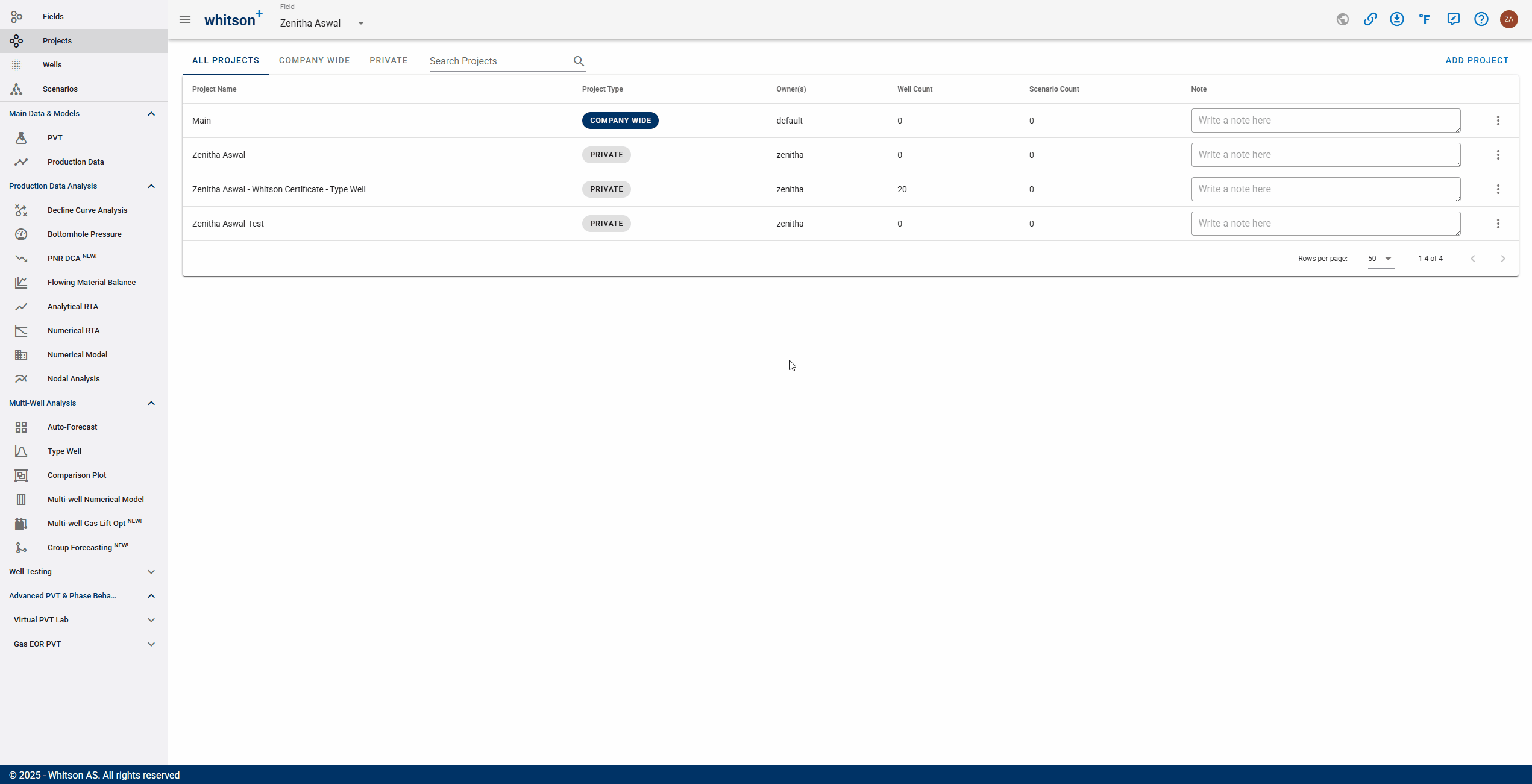
- Go to the Projects module in the navigation panel.
- Click ADD PROJECT up to the right.
- Name the project "Your Name - Whitson Certificate - Nodal Analysis".
- Click SAVE.
- All steps are shown in the .gif above.
1.3. Upload Well Data
- Click MASS UPLOAD up to the right.
- In the pop-up window, select EXAMPLES
- Search for Nodal Certificate Wells and click UPLOAD
- You can also download the data from →→ here ←← and upload the data in your project dropping the data file into the MASS UPLOAD frontend.
- All the data will be uploaded into the project. You can then close the Mass Upload pop-up window.
- All steps are shown in the .gif.
2. Well 1: Nodal Analysis - Completion Design Sensitivity
SPE-DATA-REPOSITORY-DATASET-1-WELL-37-PHEASANT
We will start with a dry gas well, with little water production. In reality, this is the closest we will get to a "single-phase" flow problem. It is a great place to start the learning curve for unconventional well performance.
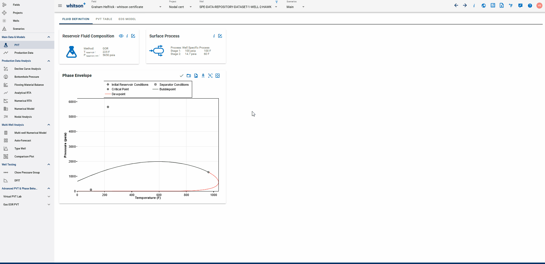
2.1. PVT
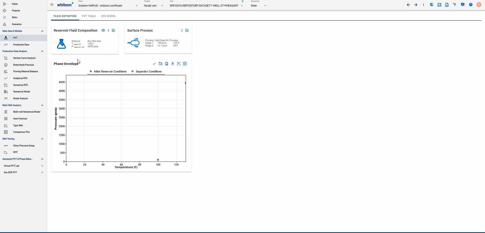
2.1.1. Reservoir Fluid Composition
- Go to the PVT module in the navigation panel.
- Open the Reservoir Fluid Composition Input Card
- Click SAVE.
- Check the predicted fluid composition by clicking the "eye icon".
- All steps are shown in the .gif above.
2.1.2. PVT Table
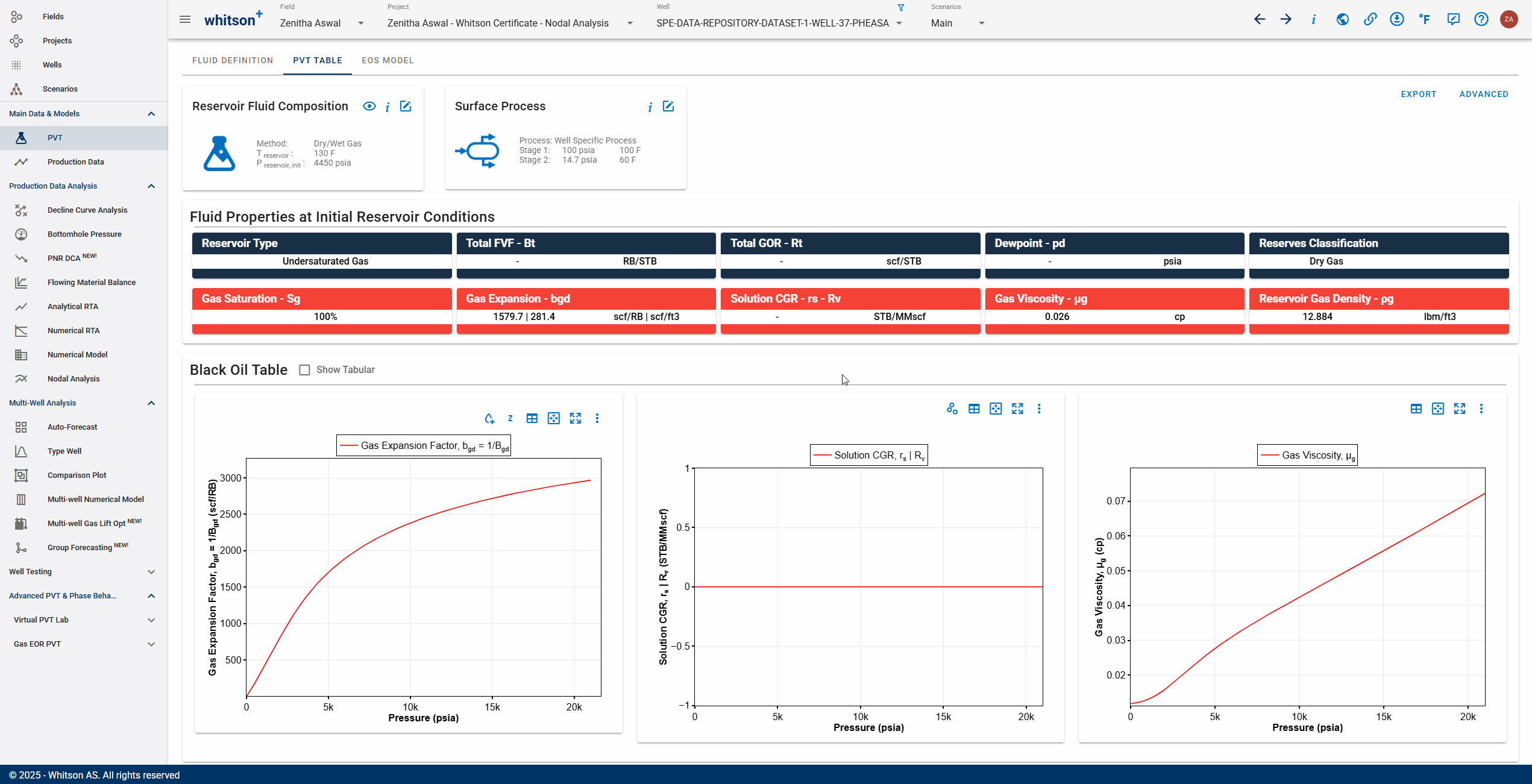
- Go to the PVT TABLE tab.
- Click EXPORT up to the right.
- Click EXCEL in the dropdown menu to download the table to excel.
- We'll not use this table, this is just to show you how this is done.
- This table represents the PVT that will be used for this well.
It's done automatically - so just sit back and relax (: - All steps are shown in the .gif above.
2.2. Production Data
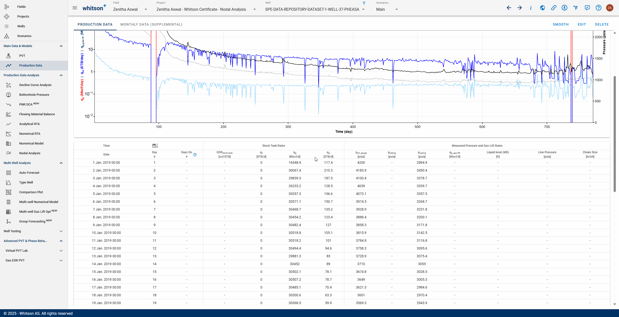
- Go to the Production Data module in the navigation panel.
- Click EDIT up to the right.
- Change the first measured gauge pressure to 4200 psia.
- Click SAVE.
- Does this well have tubing installed?
This section is meant to show you how you can manually edit the production data in case that is needed. In reality, one would not need to edit or delete the production data in most cases.
You can always smooth the data using the SMOOTH button on the top-right to make temporary adjustments to the rate profile.
2.3. Bottomhole Pressure Calculations
2.3.1. View Wellbore Configuration Data
The data for these wells has already been uploaded, so this is just for information.
Potential changes would be made in this view (if any).
- Go to the Bottomhole Pressure module in the navigation panel.
- Open the Well Data input card.
- The (1) Well Deviation survey can be plotted by clicking the icon next to the "Deviation Survey" text.
- Click the (2) Well Data tab. Note that the well is currently missing a tubing, so the well is flowing up the casing and accordingly, the flowpath is casing.
- Click SAVE.
- All steps are shown in the .gif above.
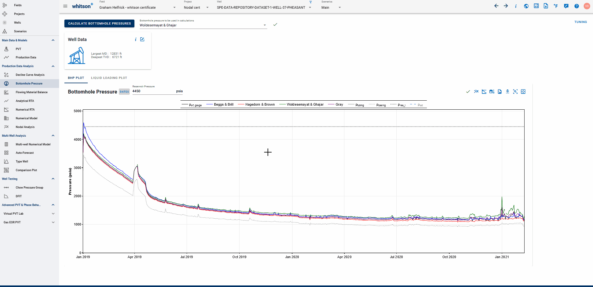
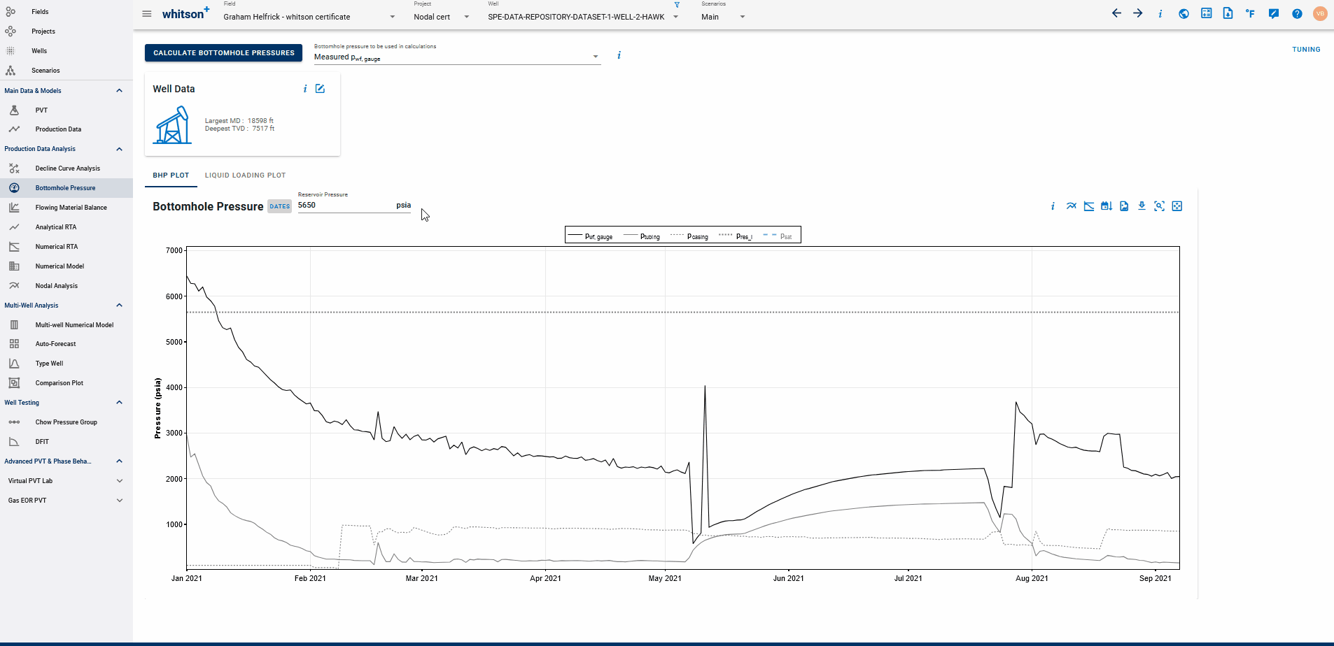
2.3.2. Calculate Bottomhole Pressures
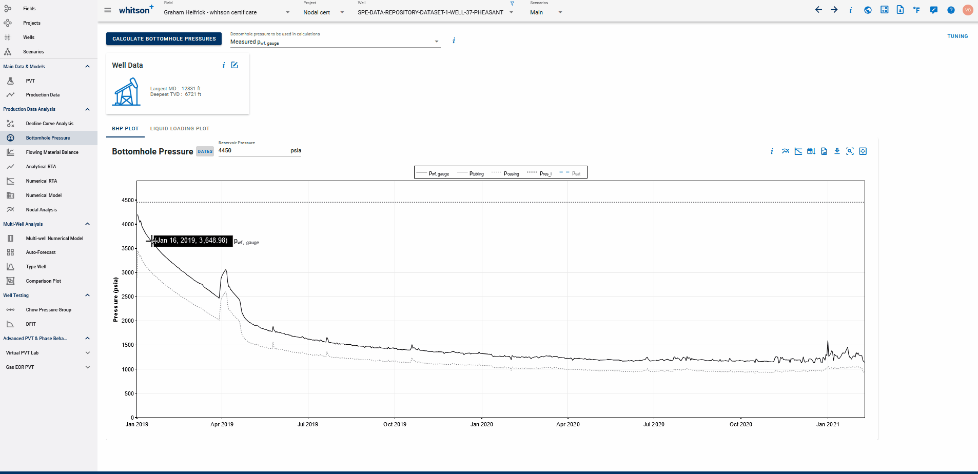
- Click the CALCULATE BOTTOMHOLE PRESSURES button.
- This will run the calculation for four different BHP correlations at the same time.
- Select Woldesemayat and Ghajar as the "Bottomhole pressure to be used in calculations".
- The dropdown menu can be found right next to the CALCULATE BOTTOMHOLE PRESSURES button.
- The selected BHP is used everywhere in the software where BHPs are required (PNR DCA, FMB, RTA, Numerical Model, Nodal Analysis).
- All steps are shown in the .gif above.
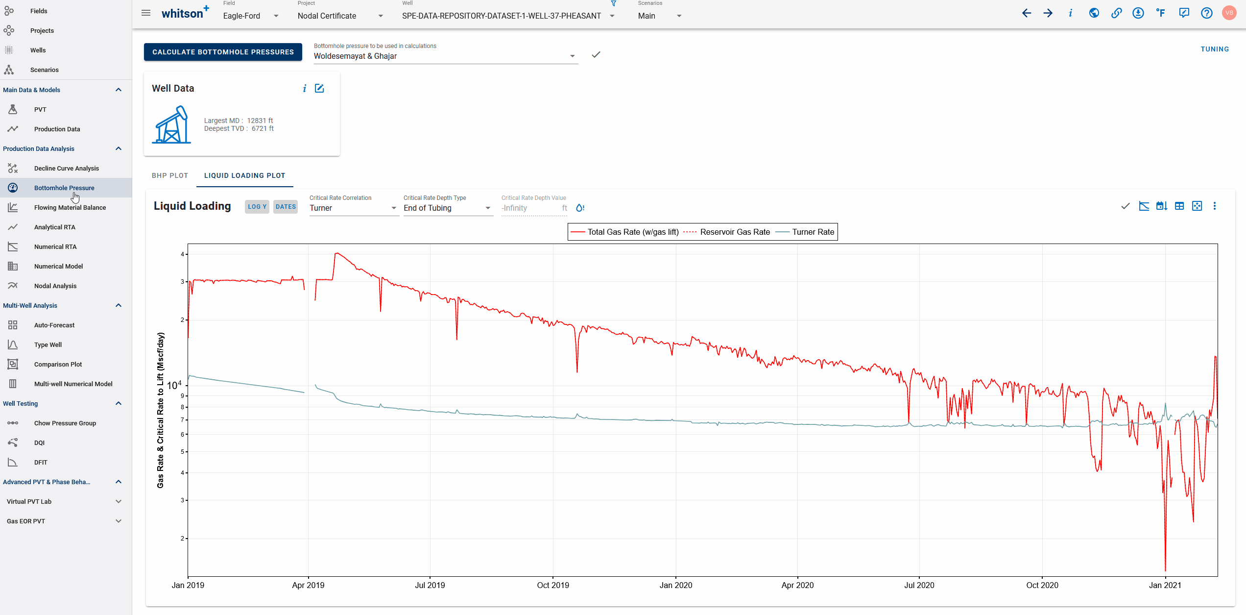
2.3.3. Liquid Loading
- Click the Liquid Loading tab of the Bottomhole Pressure feature.
Here, you can compare your actual gas rates to the required critical gas rates to deliver gas through the current wellbore configuration without any liquid loading issues. - The critical rate is computed at the end of tubing using the Turner correlation by default.
You can always change the correlation to use and the depth at which these critical rates are reported for. - Does it look like the well is going to be liquid loaded?
You always want to ensure that the actual gas rates from the well are higher than this crtical rate - this is a commonly used diagnostic for gas wells.
2.4. Nodal Analysis
2.4.1. Create an IPR and VLP
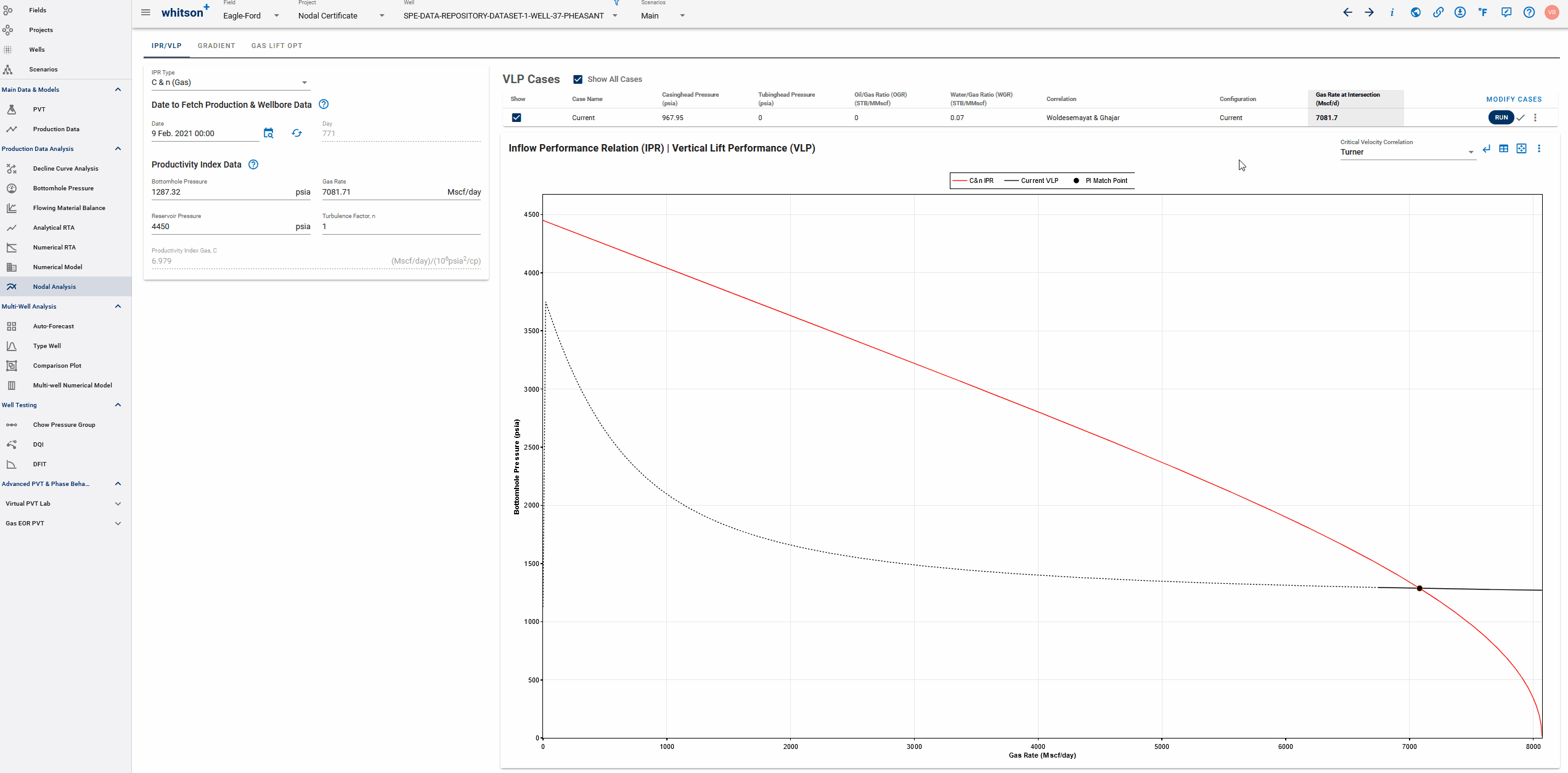
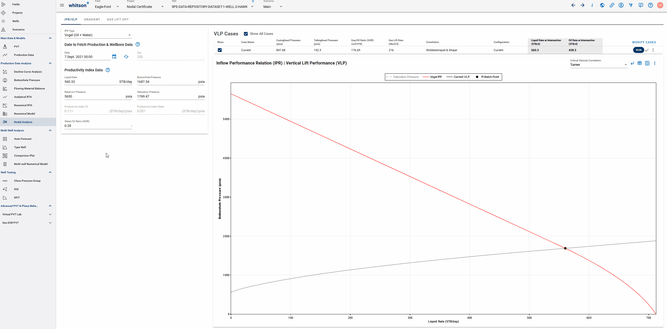
- Click Nodal Analysis from the navigation panel on the left.
- Choose a date to create an IPR, VLP curve - for this case, we'll choose the most recent date which is also the default selection for generating an IPR.
Note
This automatically pulls the bottomhole pressure, reservoir pressure, gas/liquid rate and the wellbore configuration in use for the chosen date and creates a VLP case for that date. Note that this case should use the same correlation as chosen above (Woldesemayat and Ghajar) for BHP.
IPR type has two choices:
- C & n IPR or the backpressure equation - default for Gas wells
- Vogel IPR - default for oil wells.
For the reservoir pressure, you have the following options for the source of the average reservoir pressure for the chosen date:
- Multiphase Flowing Material Balance (MFMB) or dry gas FMB,
- Numerical model history match
- Initial Reservoir Pressure - If none of these analyses have been performed, the initial reservoir pressure is assumed to be the average pressure by default.
In this case, we'll just skip the additional analyses and work with defaults - the initial reservoir pressure of 4450 psia.
This also automatically runs the case and generates the VLP, with solid and/or dotted lines, where, the dotted section of the VLP indicates the operating conditions with the well configuration in use that will likely cause liquid loading in the well - based on the critical rates.
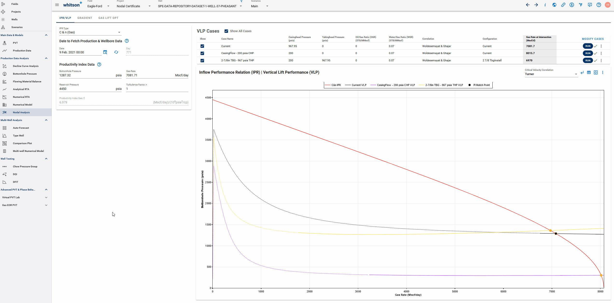
The operating point (given by the intersection of the IPR and VLP from the wellbore configuration on the chosen date) is represented with a black marker, this represents the current gas rate and bottomhole pressure deliverable by the well configuration in use, as of the chosen date. The rate at the point of intersection is reported in the case table.
This shows that we're nearly at the point where the well will quickly start liquid loading if we continue producing it via the casing. Can we prevent this by simply lowering the casing pressure of this well or is it about time we consider installing tubing? Let's find out!
2.4.2. Adding a New VLP Case
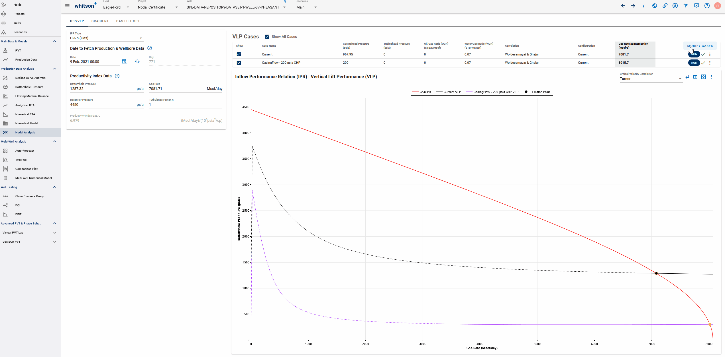
Case 2: Add a new case - Lower Casing Head Pressure
- For our first test, let's see the effects of lowering the casing pressure. No need for any changes to the well configuration here, we'll just rerun the VLP for a lower casing pressure and gather the intersection with IPR to see the resulting rates.
- You can add a new case by clicking the Modify Cases button. Replicate the first row into the second row with a quick copy-paste as shown above.
- Name the case "CasingFlow - 200 psia CHP" and modify the Casing Pressure to 200 psia. Click SAVE.
- The new case is run automatically, you should have two VLP curves for the two cases in the VLP cases table.
Note
Note how the intersection between the IPR and VLP shifts, representing a higher well deliverability in terms of gas rates with bottomhole pressure lowered further. This also delays liquid loading significantly because the new VLP is liquid loaded at much lower gas rates, down to about 3.2 MMscf/D.
2.4.3. Test Alternate Operating Strategies
Question
Instead of lowering the casing head pressure, what if we installed tubing in the well?
To run such a comparison, we need to repeat the steps above - each time, we add a new well configuration, enter the relevant wellhead pressure and other input and create a VLP case.
Let's build 2 additional VLP cases to compare installing tubing vs lowering casing head pressure:
Case 3: Add a New Well Configuration - Add Tubing to the Configuration
- Click Modify Cases and ADD/EDIT WELLBORE CONFIGURATION to add a new configuration.
- Any modification compared to the "Current" wellbore configuration (which is the active configuration for the selected date from the Bottomhole Pressure section) will need to be saved with a unique name. Let's call this configuration "2 7/8 TbgInstall".
- You can use the tubing tables to add 2 7/8", 6.4 ppf tubing OD and ID up to 6500 ft (Tubing depth in MD) and choose the "Tubing" flowpath.
- Click SAVE.
- In the VLP cases table, add a new VLP case - call it "2-7/8in TBG - 967 psia THP".
- Use a tubinghead pressure of 967.95 psia and a casinghead pressure of 200 psi.
- Make sure to activate the new well configuration (2 7/8 TbgInstall) for this case in the Configuration column.
- Click SAVE. See steps in the GIF above.
Note
The Configuration column dictates which configuration will be used to calculate the VLP - we need to choose this saved configuration here for the appriopriate VLP case to ensure that this case uses the saved configuration to calculate BHP instead of the current configuration.
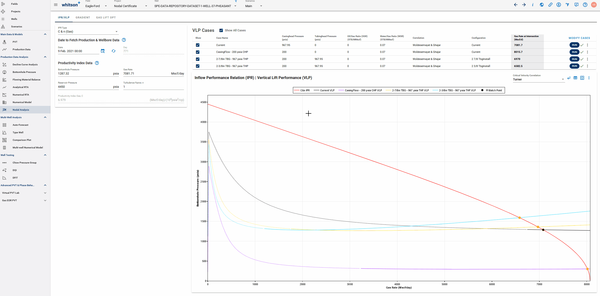
Case 4: Add a New Well Configuration - Let's Try a Different Tubing Size
- Click Modify Cases and ADD/EDIT WELLBORE CONFIGURATION to add a new configuration.
- Let's call this configuration "2 3/8 TbgInstall".
- You can use the tubing tables to add 2 3/8", 4.6 ppf tubing OD and ID upto 6500 ft (Tubing depth in MD) and choose the flowpath as Tubing. Click SAVE.
- Add another VLP case - call it "2-3/8in TBG - 967 psia THP".
- Use a tubing head pressure of 967.95 psia.
- Choose the newly created configuration "2 3/8 TbgInstall" using the dropdown in the Configurations column.
- Click SAVE. All these VLP cases should calculate automatically and plot on the IPR-VLP plot. The VLP cases table summarizes the cases with the gas rate at intersection.
Notice how the smaller tubing has a higher frictional pressure drop so it results in slightly lower rate but increased BHP and a much more delayed liquid loading.
Note
Since we added tubing to the configuration and the flow is up the tubing, the casing pressure used is no longer relevant to the VLP and only the tubing pressure will make a difference. For the purpose of continuity, the tubing pressure used above is the casing pressure that the well was being produced with, on that chosen date.
All the steps are shown in the GIFs above.
2.4.4. Saving VLP Cases, Viewing/Editing Wellbore Configurations in Use
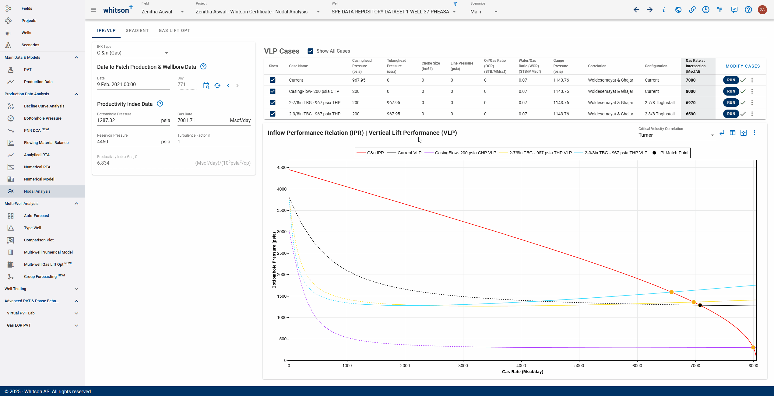
- All the cases added to the VLP cases table are automatically saved. You can work on other things and when you navigate to nodal analysis for this well, it will be exactly as you left it previously.
- To compare all or few these cases, you can toggle the cases on/off by clicking on the legend entry.
- To adjust or view the wellbore configuration in use, click Modify Cases and ADD/EDIT WELLBORE CONFIGURATION. Select the configuration you want to edit by choosing this configuration from the dropdown here. Click SAVE to update this saved configuration.
All these steps are shown in the GIF above.
2.4.5. Conclude
We used nodal analysis to see if this gas well can be prevented from liquid loading in the near future by adjusting the operating conditions:
- You can modify the current case by changing the date input on the left, as the changes in the current case can not be made in the ADD/EDIT WELLBORE CONFIGURATION.
- Click on the date and a screen will appear. You can adjust the date by moving the vertical dashed line to the desired date or manually type the days.
- Click Save. You can see the changes in the current case.
Bonus questions
- Which operating conditions offer the highest incremental rate? Does this prevent liquid loading?
- Which configuration would you pick to sustainably prevent liquid loading for the longest time and why?
You can include these answers along with your certificate project submission below.
3. Well 2: Nodal Analysis - Gas Lift Optimizer
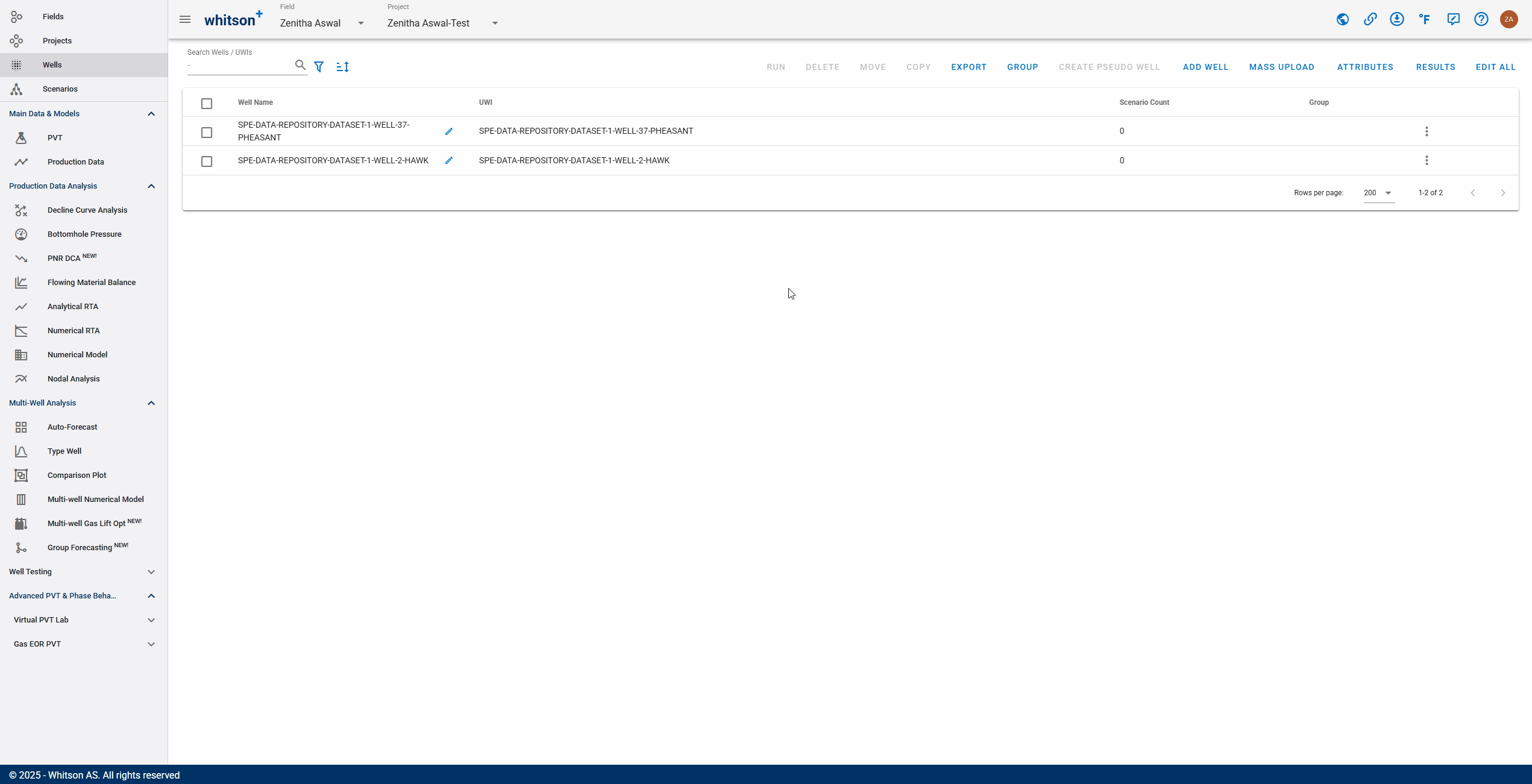
This workflow will be done on different well in the same project called "SPE-DATA-REPOSITORY-DATASET-1-WELL-2-HAWK"
This is an Eagleford black oil well. The preliminary steps to conduct this analysis include initializing PVT, updating the wellbore configurations to include gas lift valve details, and calculating BHP and viewing gas injection depths vs time.
The rest of the workflow involves using Nodal analysis and specifically the gas lift optimizer, where we will examine the effects of altering gas lift injection rate on produced oil and see the optimal gas injection rate to maximize the same. We will also conduct a lookback by picking a date when the gas lift injection was much lower than this optimum - to see potential upside of increasing the lift rate sooner.
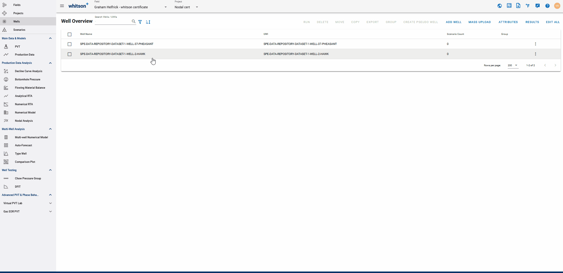
- Click Wells from the navigation panel on the left.
- Click the SPE-DATA-REPOSITORY-DATASET-1-WELL-2-HAWK
3.1. PVT
- Navigate to the PVT section and click the edit icon on the Reservoir Fluid Composition card. Note that the initial GOR was preloaded from the mass upload for this well.
- Click Save. This generates the fluid composition and the relevant black oil tables.
3.2. Bottomhole Pressure Calculations
3.2.1. Correcting Wellbore Configurations - Adding Valve Details
- Go to the Bottomhole Pressure module in the navigation panel.
- Open the Well Data input card.
- Click the (2) Well Data tab. Note that there is only one configuration here since the gas lift calculation is only activated for the days when there are gas lift injection rates in the data. For the days that do not have gas lift rates, the BHP calculation simply assumes tubing flow with no artificial lift.
Choose 'Valves' for 'Gas Lift Configuration' and click the edit icon to enter the valve details (depths, opening and closing pressures) as follows:
| Valve MD (ft) | PSO (psia) | PSC (psia) |
|---|---|---|
| 1500 | 1158 | 982 |
| 3000 | 1120 | 950 |
| 5000 | 1060 | 870 |
| 7000 | 1015 | 834 |
Click Save to save the valve details and click the Save button again to save this wellbore configuration. All these steps are shown in the GIF above.
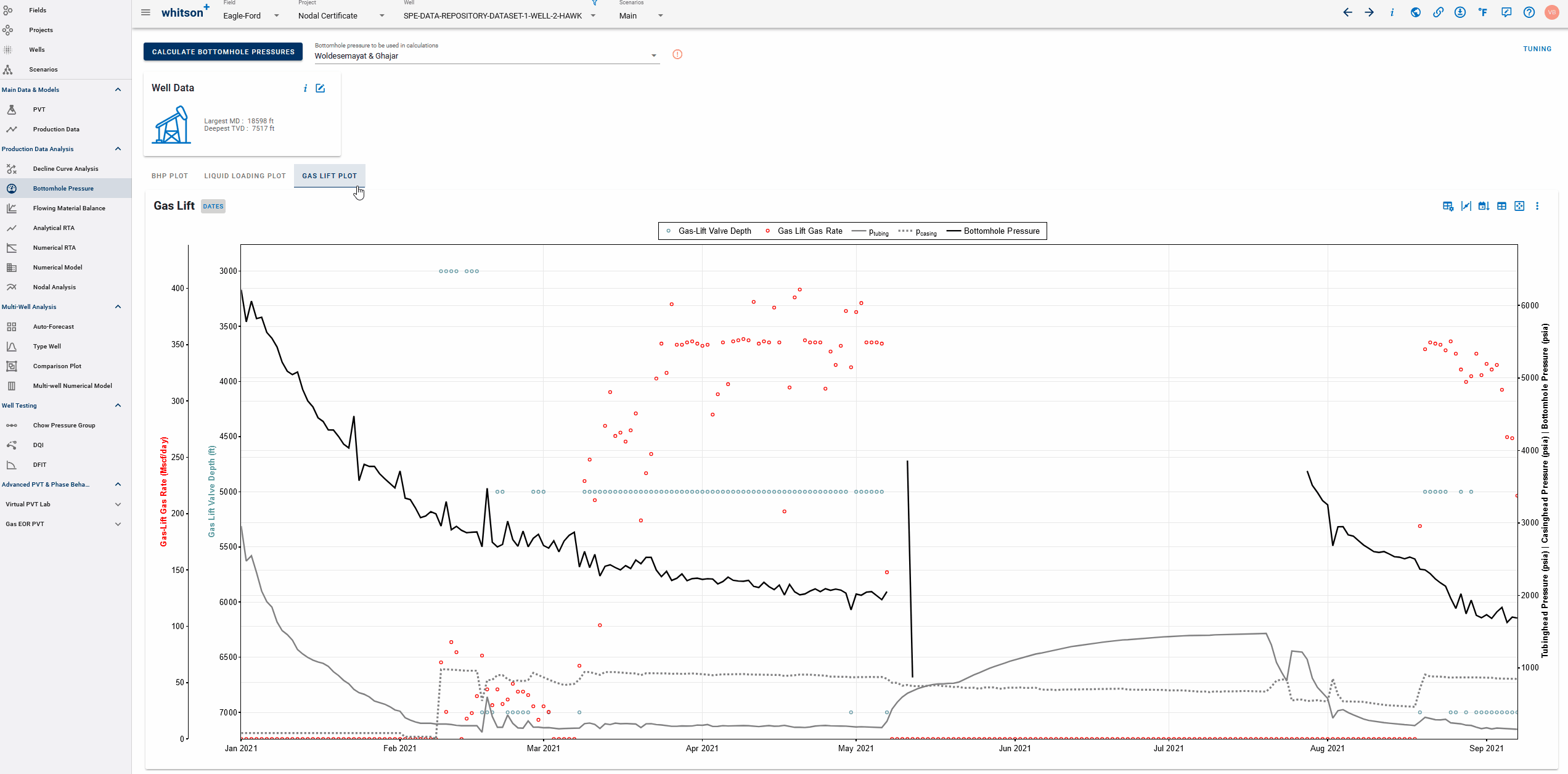
3.2.2. Calculate BHP and View Gas Injection Depths
- Click the CALCULATE BOTTOMHOLE PRESSURES button.
- This will run the calculation for four different BHP correlations at the same time. For gas lift wells, this also calculates the operating valve (i.e. the valve that the lift gas is injected into - depending on the casing and tubing pressures) for the gas lifted portion of the well history.
- Select Woldesemayat and Ghajar as the "Bottomhole pressure to be used in calculations".
- The dropdown menu can be found right of the CALCULATE BOTTOMHOLE PRESSURES button.
- The selected BHP is used everywhere in the software where BHPs are required (PNR DCA, FMB, RTA, Numerical Model, Nodal Analysis).
- Click the Gas Lift Plot to view the gas injection depths vs time for the given gas lift design - just double-click the 'Gas-Lift Valve Depth' in the plot legend to isolate this data on the plot. You can also enable gas lift valve depths to see where the installed valves are located in the wellbore.
Notice how the gas lift is injecting shallow at the beginning and eventually injects into the deepest valve at later time with increased rates so there might be potential for further optimization.
3.3. Optimizing Gas Lift Rates
Why optimize gas lift?
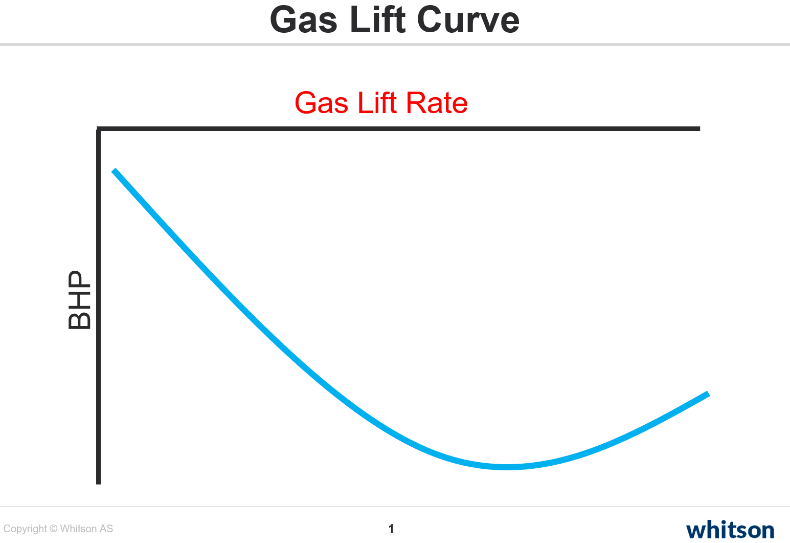
Gas lift is a useful form of artificial lift that works by primarily lowering the density of fluid column in the wellbore, effectively reducing the hydrostatic pressure. This indirectly increases the pressure differential (drawdown) between the reservoir and the bottomhole, hence enhancing more fluids to flow or be produced.
Optimization of a gas lifted well may involve changing gas injection rate, pressure, etc. to control the gas injection depth in the wellbore and hence reduction in the bottomhole pressure. The most optimized design injects as deep as possible into the wellbore and yields the maximum reduction in bottomhole pressure.
A diminishing return can be anticipated when the design parameters are pushed to inject more gas into the wellbore. The gas injected in excess of this optimal limit has a higher frictional pressure drop in the wellbore, which in turn, yields a higher bttomhole pressure and reduces the production rate.
3.3.1. Step 1: Nodal Analysis
- Navigate to Nodal Analysis.
- Ensure that the most recent date is selected for the IPR - that should be the default. This pulls in the current gas lift configuration in place and the associated BHP, rates available for generating the IPR.
- This automatically generates a VLP curve for the current conditions and the intersection represents the current operating point with the associated gas lift rates and wellhead pressures on that day.
We could manually add multiple VLP cases with different lift gas rates here to find the most optimal gas-lift injection rate that lowers the BHP and maximizes the produced liquid rates.
Instead, we'll skip this sensitivity analysis and directly use the Gas lift Optimizer (which does that for you) below.
3.3.2. Step 2: Gradient Calculator
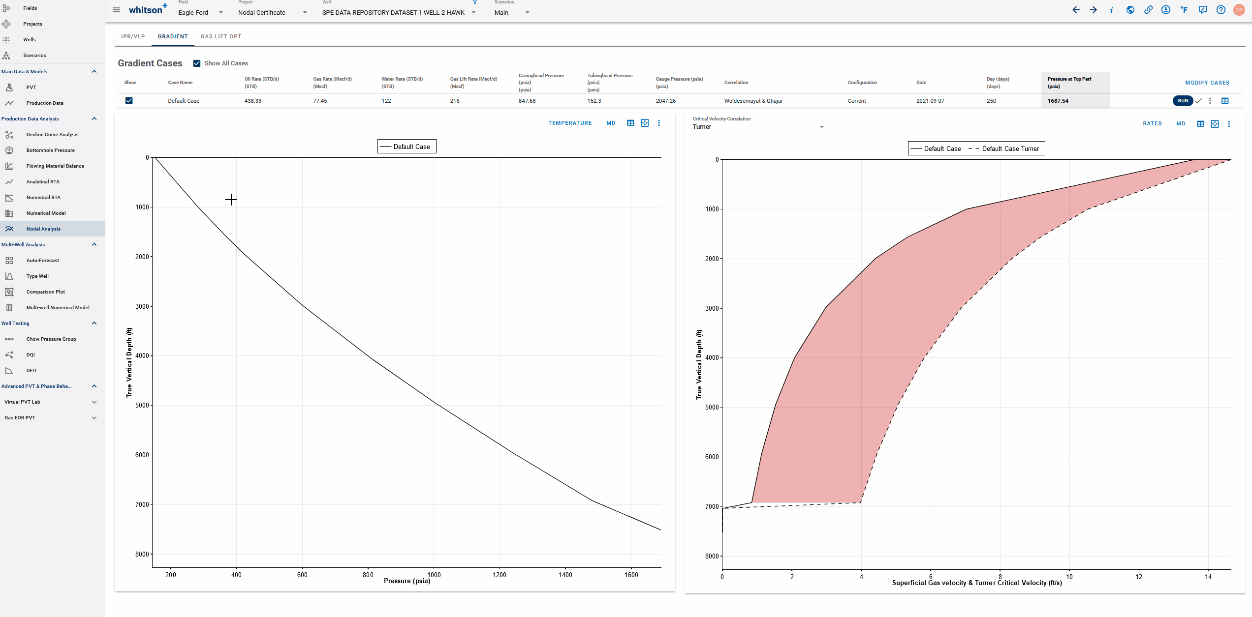
- Switch over to the Gradient Calculator tab on the top. The conditions on the selected date in IPR-VLP is automatically the first, default case.
- Gradient cases are listed at the top, you can build alternate cases by clicking Modify Cases as shown in subsequent steps.
- Click RUN to generate the pressure traverse curves i.e. pressure drop through the wellbore down to the MD/TVD. The case we just ran plots the pressure drop in the wellbore for the chosen date in IPR, along with gas rates and velocities - actual and critical to see the length of the wellbore under likely risk of liquid loading.
- Click summary button to see the complete set of calculated values vs depth, expected flow regimes in the pipe etc.
- You can switch between pressure vs TVD and pressure vs MD.
Why does pressure vs MD look counter-intuitive?
To answer this question, we need to take a look at the deviation survey to see the toe and the heel of the lateral:
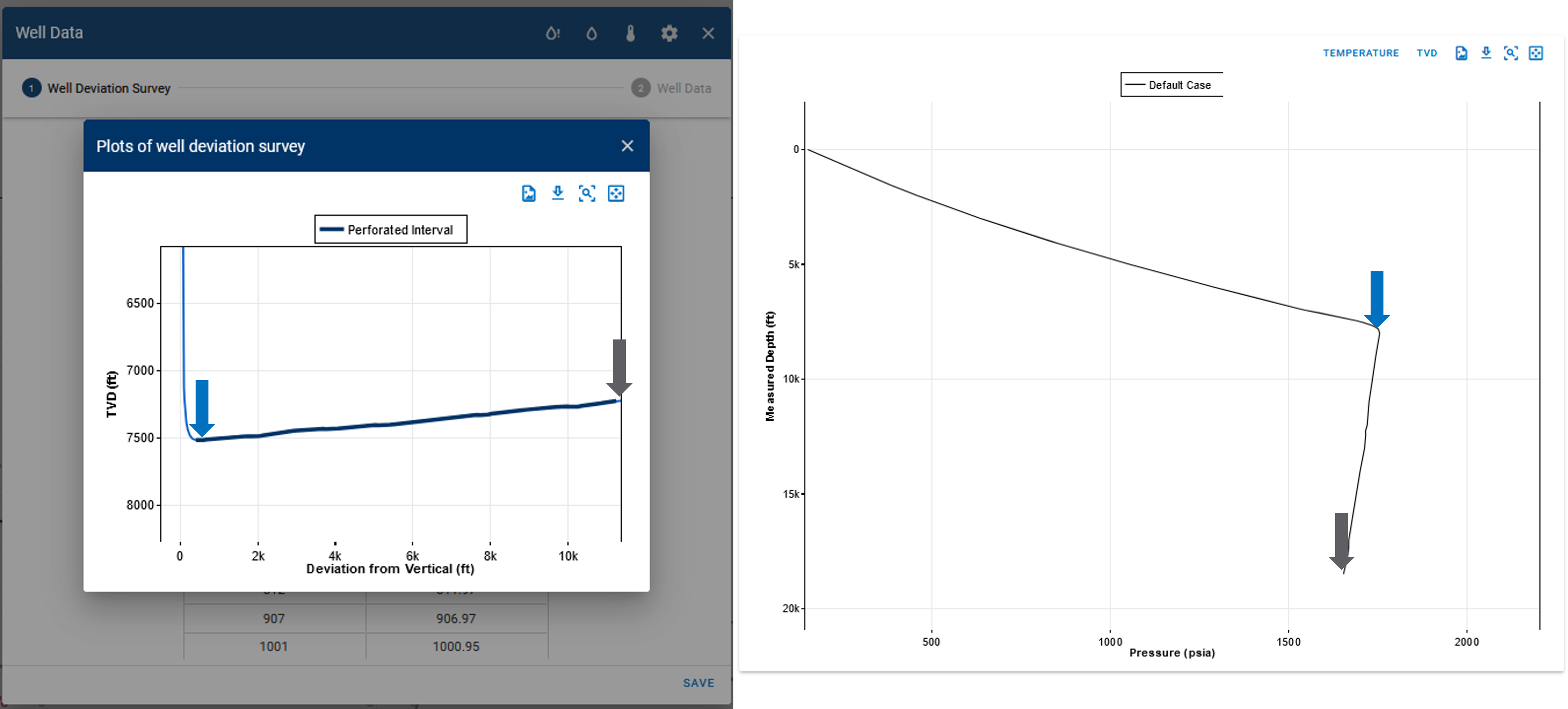
The well construction is toe-up, such that the toe of the lateral is shallower than the heel of the well lateral. This creates a lower pressure at the toe and higher pressure at the heel which causes this shape in pressure vs MD.
3.3.3. Step 3: Gas Lift Opt
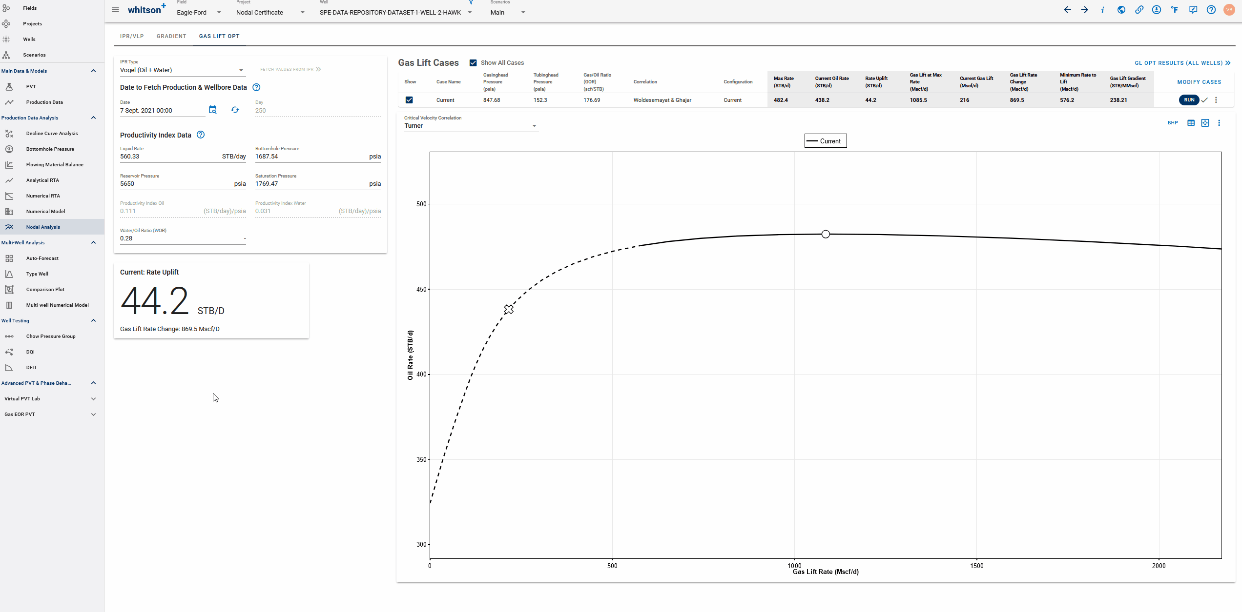
- Switch over to the Gas Lift Opt tab on the top.
- This plot shows you the oil rate yield curve, where the incremental oil recovery with incremental increase in gas injection rate can be plotted based on the IPR/VLP for that chosen date.
- The plot shows the current operating point with an X marker and the most optimal operating conditions with the circle marker. The curve itself shows that the oil recovery reduces with an increase in gas lift rate beyond the optimal point.
- You can add additional cases by clicking MODIFY CASES to adjust parameters such as tubing and casing pressure. This also allows for the option to modify the wellbore configuration to generate the gas lift optimization curve for alternate strategies (such as injecting via the tubing or modified gas lift valve depths)
Notice that this analysis recommends increasing the gas injection rate by ~896 Mscf/D to about 1112 Mscf/D to produce an additional 50.6 STB/D. This additional recovery can be achieved, at times with minor modifications to gas lift wells.
On the flip side, we can also see the impact turning off gas lift - the point where the curve intersects the y-axis (lift gas injection rate = 0) represents the achievable oil rates with the same wellbore configuration if the gas injection was completely turned off. From the plot here, we can see that the well would still make 320 STB/D with no lift-gas injection - although with potential liquid loading issues! The dashed/solid in the curve also shows the minimum gas lift rate to lift without these liquid loading issues - you can infer this critical rate from the table at the top which summarizes key results.
3.4. Lookback - When the Gas Lift Rate was Lower
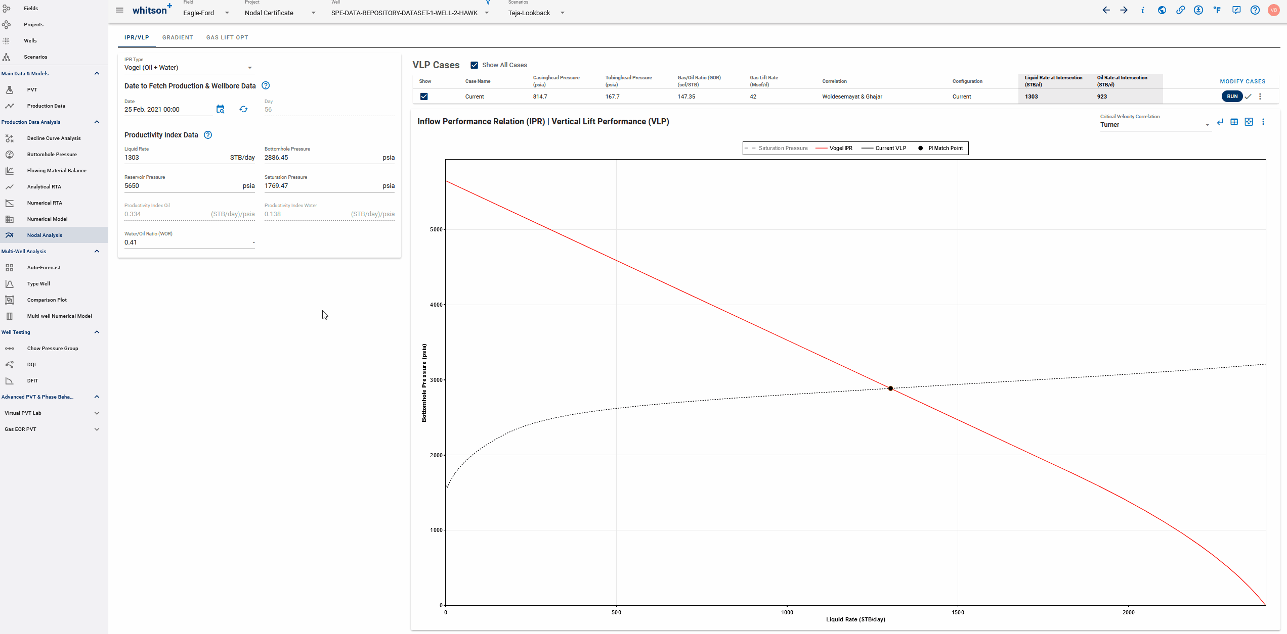
3.4.1. Lookback - IPR/VLP
- Navigate back to IPR/VLP tab and add a new scenario, let's call it "Lookback"
- Pick 25th February 2021 (or day 56 in the well history) to calculate the IPR and VLP for that date - The reason we choose this date for a lookback is because we were injecting much lower gas-lift rates, so there should be a much higher margin for optimization.
- This action will automatically populate the "Current" case with conditions from day 56.
- Now, navigate back to "Main" scenario and open MODIFY CASES. Copy all the input values from the "Current" case in the table.
- After copied these values, return to "Lookback" scenario, open MODIFY CASES, and create a new case below "Current" case, called it "Lookforward". Paste the previously values copied from "Main" scenario.
Based on "Lookback" IPR, the intersection of a GL rate = 42 Mscf/d (Current) results in higher bottomhole pressure and lower oil rate, indicating not an optimal gas-lift injection compared to a GL rate = 216 Mscf/d (Lookforward).
Creating a scenario in whitson+
When you click on "Add a new scenario" from anywhere in the software (Dropdown right up top or the Scenarios page), you take the current scenario you are on (i.e.all the analyses/interpretation/input you have in there) and create a copy. All scenarios refer to the production data in the 'Main' scenario - so you will not be allowed to edit the production data from any of the scenarios (other than 'Main') - but you can edit all other input (including smoothing on the production data) without affecting any other scenario.
Another pro-tip: If you want to create a copy of a particular scenario, first navigate to that scenario (by clicking on it from the dropdown) and then click the "Add scenario" button. Creating a scenario always copies everything from the scenario it is created from.
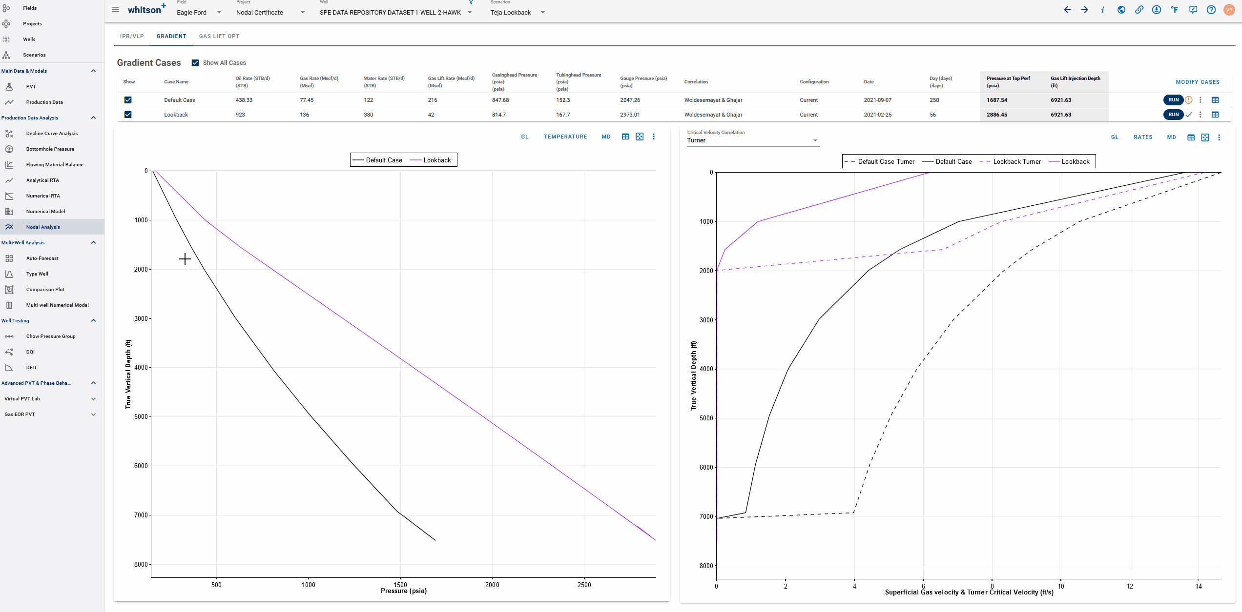
3.4.2. Lookback - Gradient Calculator
Let's run the gradient calculator for this case to confirm that this gas lift injection rate yields a much higher bottomhole pressure:
- Navigate to the Gradient Calculator tab on top.
- Under the list of Gradient Cases, Click the Modify Cases button off to the right.
- Here, instead of replacing the case we originally set up for the most recent date, we'll add a case here, let's call it "Lookback" and use the date picker in the table to select day 56 and pull all the associated values required for the table. Click SAVE.
- Automatically, your new case should be running and you should be able to see the results on the plots below these cases.
You see that the bottomhole pressure for the lookback case shows much higher bottomhole pressure at TVD compared to the most recent case. Is the pressure gradient (psi/ft) in the wellbore higher or lower for the new case we just added above?
Tip
If an orange exclamation mark appears next to the case, that means the input has changed, making the results outdated. Click RUN to recalculate.
3.4.3. Lookback - Gas Lift Optimizer
Next, we'll run the gas lift optimizer for this date, steps shown in the GIF above:
- Navigate to the Gas Lift Opt tab on top.
- Click "Fetch Values from the IPR". This ensures that the gas lift optimizer is using the appropriate data as in the IPR/VLP section.
- Notice how the gas lift optimization curve is automatically recalculated?
- The warning sign, if any, should be replaced with a green check mark when done. Time to look at the results!
It shows that the margin for improvement is much higher. If we increased the lift gas injection rate to 1522.3 Mscf/D, we have the potential to recover about 1192 STB/D instead of the 923 STB/D in oil rates - this is an increase of almost 270 STB/D!
The gas lift optimization curve also shows that the lift gas injection rate used on this date is barely effective - turning it down all the way to 0 Mscf/D, still allows the well to deliver about 900 STB/D.
3.5. Conclude
This clearly outlines the benefits of using Nodal Analysis - specifically the gradient calculator and the gas lift optimizer, in this case to improve the lift efficiencies and test alternate strategies of lift gas injection rate and pressure combinations to optimize the well deliverability.
Such analyses are invaluable to all producing wells, so we can operate them at much higher efficiency.
Bonus questions
-
If we did not have the additional gas available to inject, how would you use nodal analysis to prove that you can produce the same rate uplift without changing the current gas injection rate? What would you prefer to change in this configuration?
-
Can you prove your plan with a quick gas lift optimization calculation?
4. Done?
When you are done with your analyses, please:
- Send an e-mail to certification@whitson.com
- Make the subject: "whitson+ Nodal Analysis certificate: [YOUR NAME HERE]"
- Include the link to your project.
- If you have any notes, comments, or observations related to the exercise, feel free to share them with us. Also feedback on the user friendliness of the software is always appreciated.
After that, we'll provide some feedback on your evaluation and issue your whitson+ certificate if all looks good.
Cheers and Congratulations!