whitson⁺ - Multi-Well Numerical Model Certification

1. Introduction

Complete the steps outlined below to become a certified whitson⁺ user. It includes performing a well performance workflow for two wells with actual production data from the SPE Data Repository and creating a synthetic well to provide a Field Development Optimization analysis. Those certified have the software skills necessary to complete most well performance evaluation projects in tight unconventionals.

Need help?

Send an e-mail to support@whitson.com.

1.1. Before Starting

Make sure you have watched these three videos in the Getting Started part of the manual (click here).

• Login (1 min)
• Overview of important basics (3 min 30 sec)
• Zoom Plots (3 min)

1.2. Create a Project

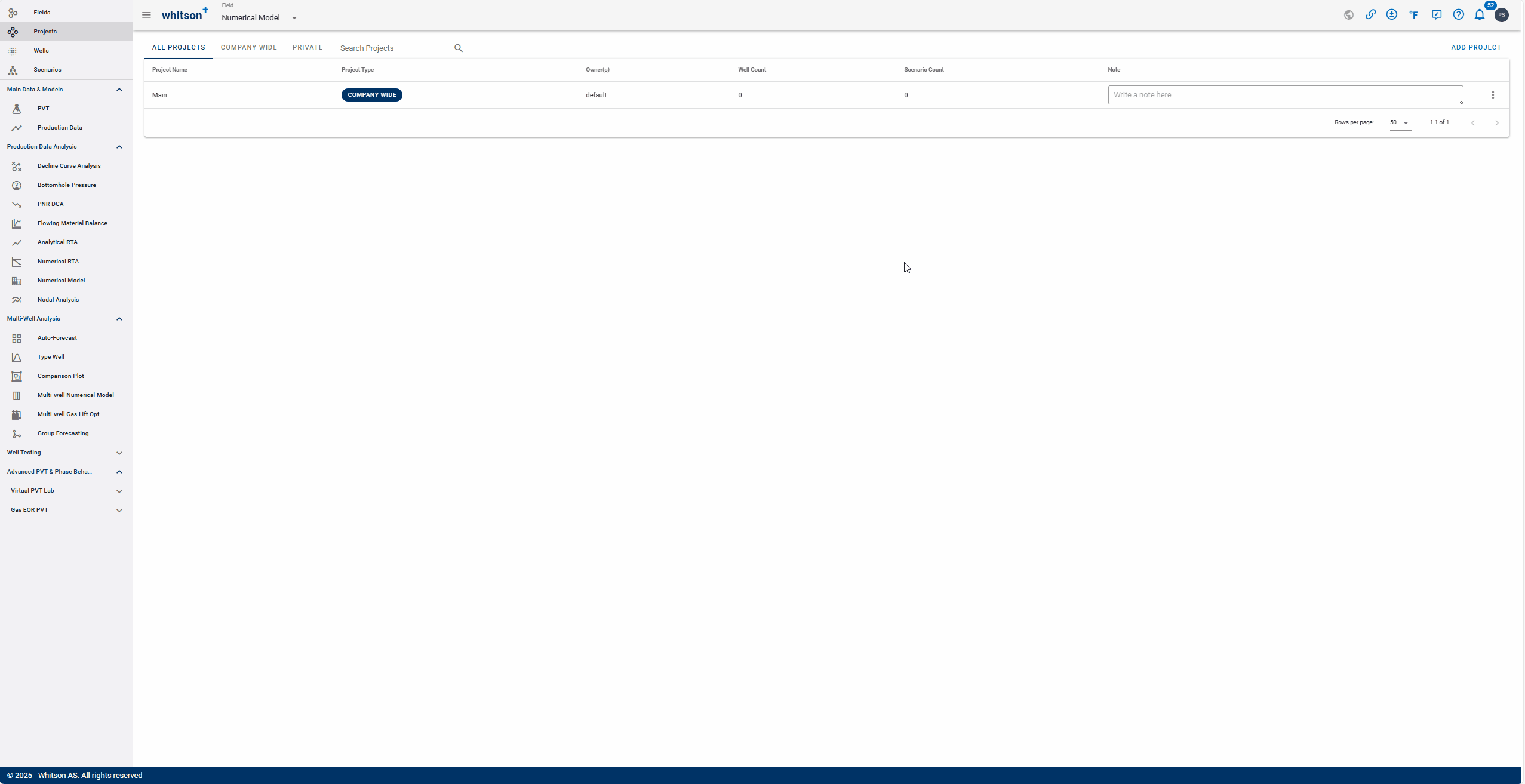
1. Go to the Project module in the navigation panel.
2. Click ADD PROJECT up to the right.
3. Name the project "your name - whitson certificate- MWNM".
4. Click SAVE.
5. All steps are shown in the .gif above.

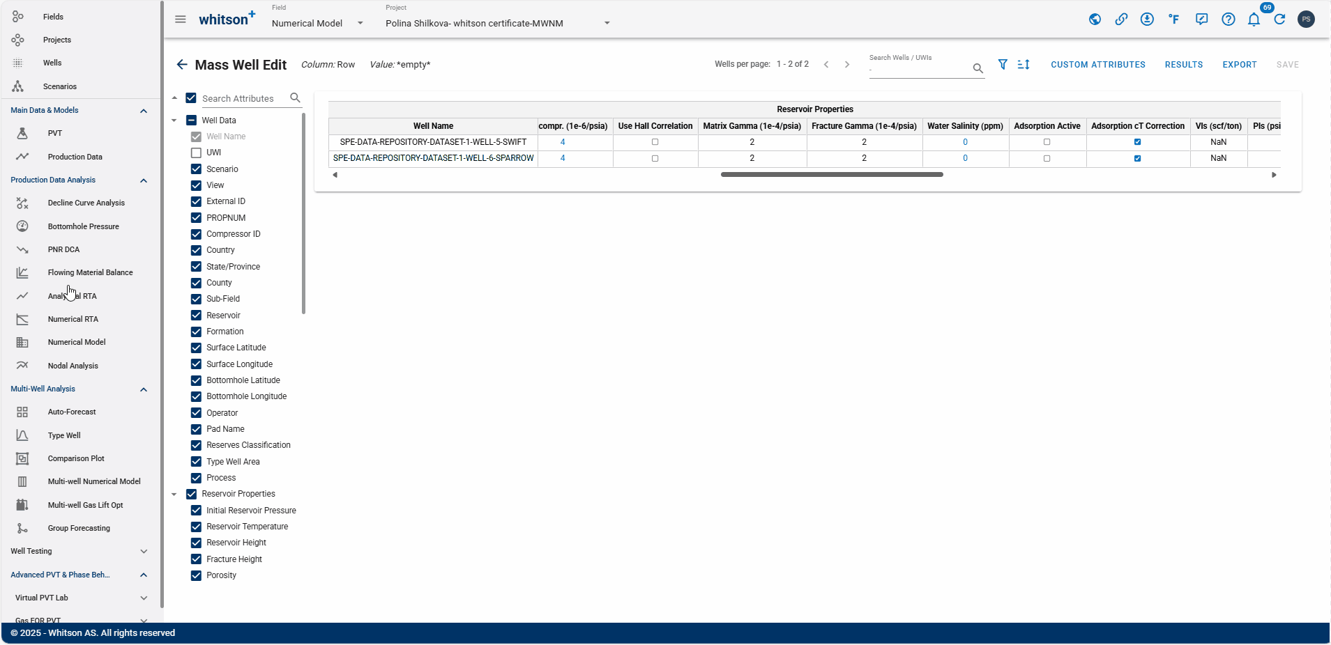
1.3 Upload Well Data

1. Click MASS UPLOAD up to the right.
2. In the pop-up window, select EXAMPLES
3. Search for Multi-well Numerical Model Certificate Wells and click UPLOAD
4. All the data will be uploaded into the project. You can then close the Mass Upload pop-up window.
5. All steps are shown in the .gif above.

1.4 PVT- Reservoir Fluid Composition

1. Navigate to the PVT module from the left-hand panel.
2. Open the Reservoir Fluid Composition Input Card
3. Initialize the fluid in the GOR method by moving the dashed horizontal line up and down to match the GOR calculated from the production data.
4. You can also input an initial GOR value in the box below. Enter 630 scf/STB.
5. Click SAVE.
6. Use the arrow at the top-right of the module to switch to the next well.
7. Repeat the same steps for the second well.
8. All steps are shown in the .gif above.

Check the predicted fluid composition by clicking the "eye icon".

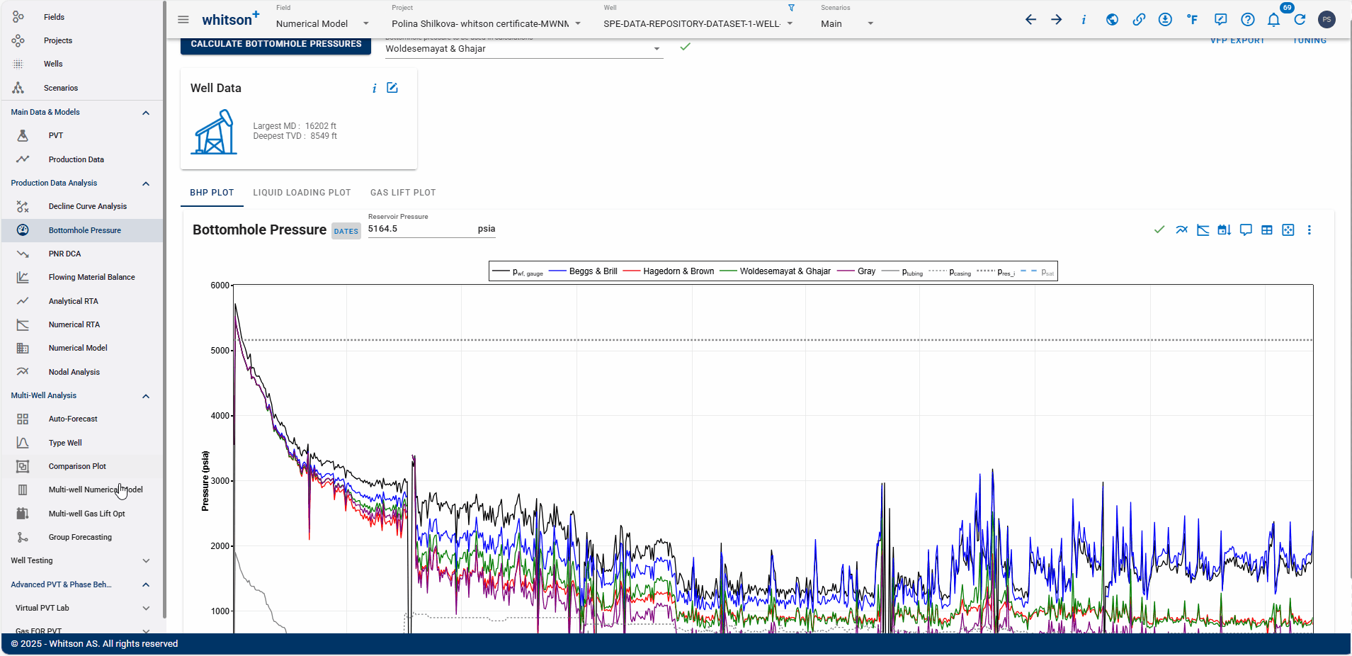
1.5 Calculate Bottomhole Pressure

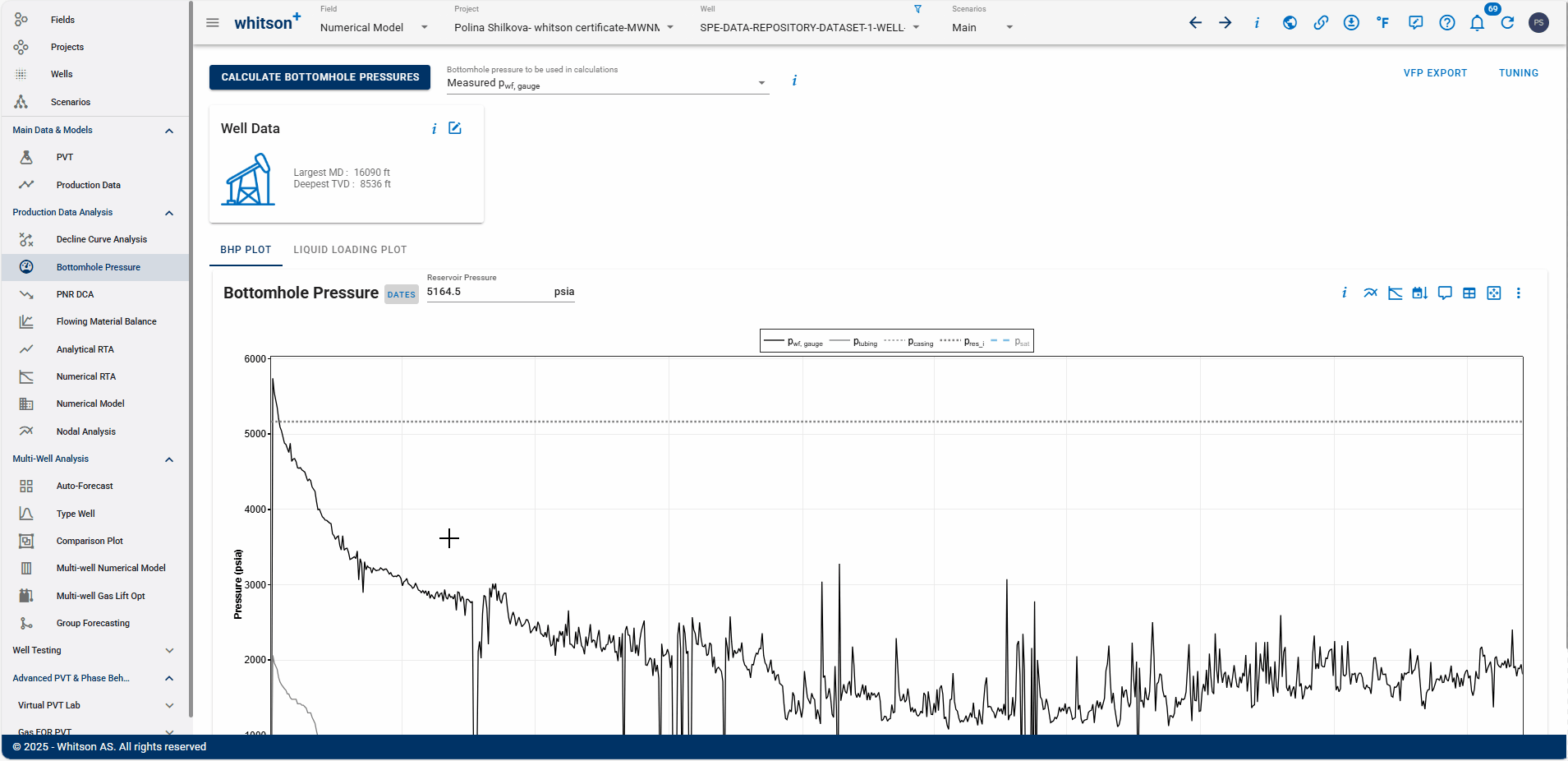
1. Go to the Bottomhole Pressure module.
2. Click CALCULATE BOTTOMHOLE PRESSURE to the upper left.
3. Change the Bottomhole pressure to be used in calculations to Woldesemayat & Ghajar.
   
4. Click CALCULATE BOTTOMHOLE PRESSURE to the upper left again.
5. Use the arrow at the top-right corner of the module to switch to the second well and repeat the steps above.
6. All steps are shown in the .gif above.

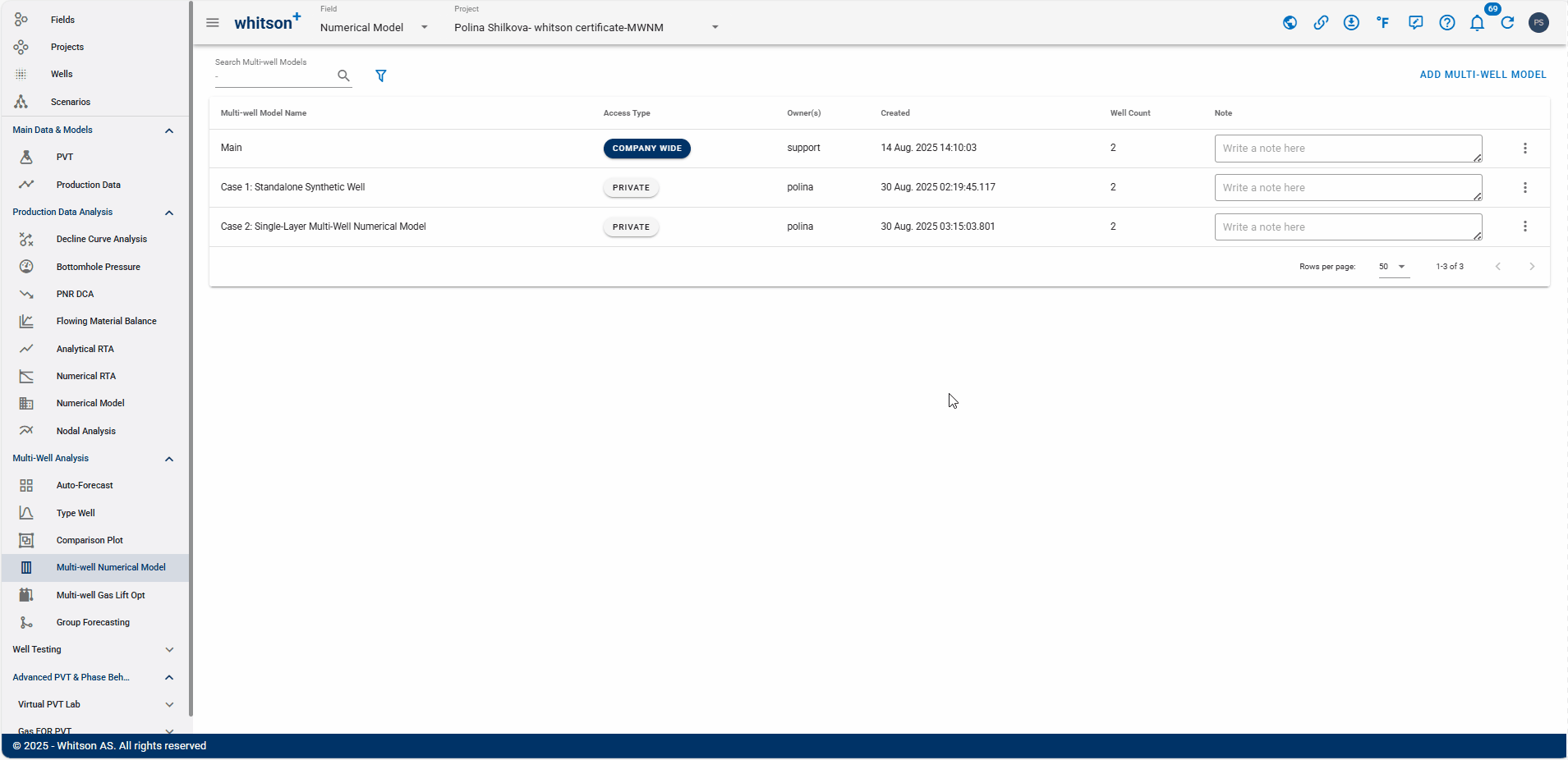
2. Multi-Well Numerical Model

The Multi-Well Numerical Model section introduces varios cases, starting from a single well and extending to complex multi-layer multi-well scenarios. By working through these exercises, users will gain insight into how well interactions, completions, and spacing choices impact reservoir performance. This workflow not only illustrates different modeling approaches but also provides a foundation for optimizing field development plans under varying geological and operational conditions.

Each case demonstrates how the numerical model in whitson⁺ can be used not only to match and simulate production, but also to test “what-if” scenarios, providing a decision-making framework for optimizing completions, well spacing, and development sequence.

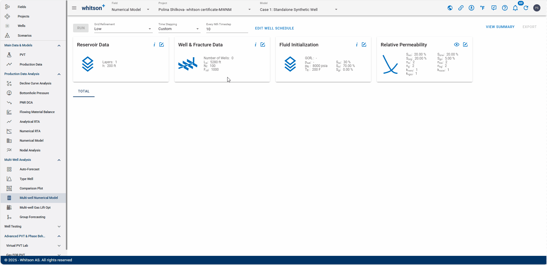
2.1 Case 1: Standalone Well

We begin with the simplest case: a single synthetic well. This serves as the foundation for learning how to set up and run a numerical model in whitson+, without the complexity of well interference. The objective is to establish baseline performance and recovery, which will serve as a benchmark when comparing multi-well cases.

2.1.1 Create a Project

1. Go to the Multi-Well Numerical Model module in the navigation panel.
2. Click ADD MULTI-WELL MODEL up to the right.
3. Provide a name and select all the wells by clicking the check box at the top of the well list (left of Well Name).
4. Click ADD MULTI-WELL MODEL.
5. All steps are shown in the .gif above.

In this case, we will use default input values to demonstrate the basic functionality of the Multi-Well Numerical Model.

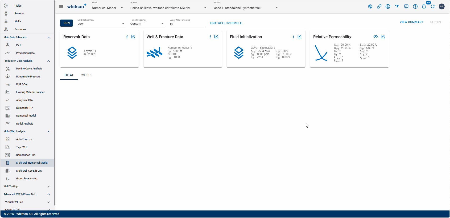
2.1.2 Reservoir Data

1. Open the Reservoir Data Input Card
   • Reservoir height \(\left(h_f\right)\), matrix permeability \(\left(k_m\right)\), matrix porosity \(\left(\phi_m\right)\), rock compressibility \(\left(c_r\right)\), fracture \(\left(\gamma_f\right)\) and matrix gamma \(\left(\gamma_m\right)\) can be entered through this data card.
2. Click SAVE.
3. All steps are shown in the .gif above.

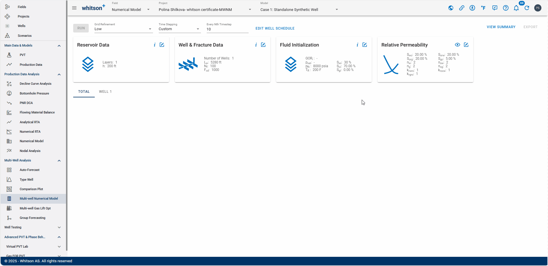
2.1.3 Well & Fracture Data

1. Open the Well & Fracture Data Input Card

   • This data card allows the user to input all relevant properties related to the well and its fractures. These include well lateral length \(\left(L_w\right)\), number of fractures \(\left(N_f\right)\), and dimensionless fracture conductivity \(\left(F_{cd}\right)\). Additionally, the user can enter well-specific properties such as distance to the next well, fracture half-length, and the perforated and fractured layers.

   Since we are creating a numerical model with a synthetic well, this well will not be linked to a specific well within the project.

2. Change the Fracture Halp Length from 400 to 300.

3. Make the Distance to Next Well of 3000.
4. Click SAVE.
5. All steps are shown in the .gif above.

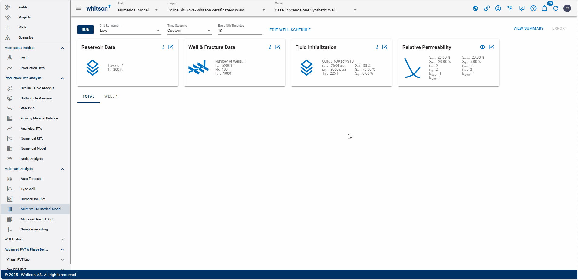
2.1.4 Fluid Initialization

1. Open the Fluid Initialization

2. Click on PVT from the well and select 5 SWIFT to assign PVT information to the synthetic well.

   In this tab, users can input initial GOR \(\left(R_{ti}\right)\), initial water saturation \(\left(S_{wi}\right)\) and initial reservoir pressure \(\left(p_i\right)\).

3. Click SAVE.

4. All steps are shown in the .gif above.

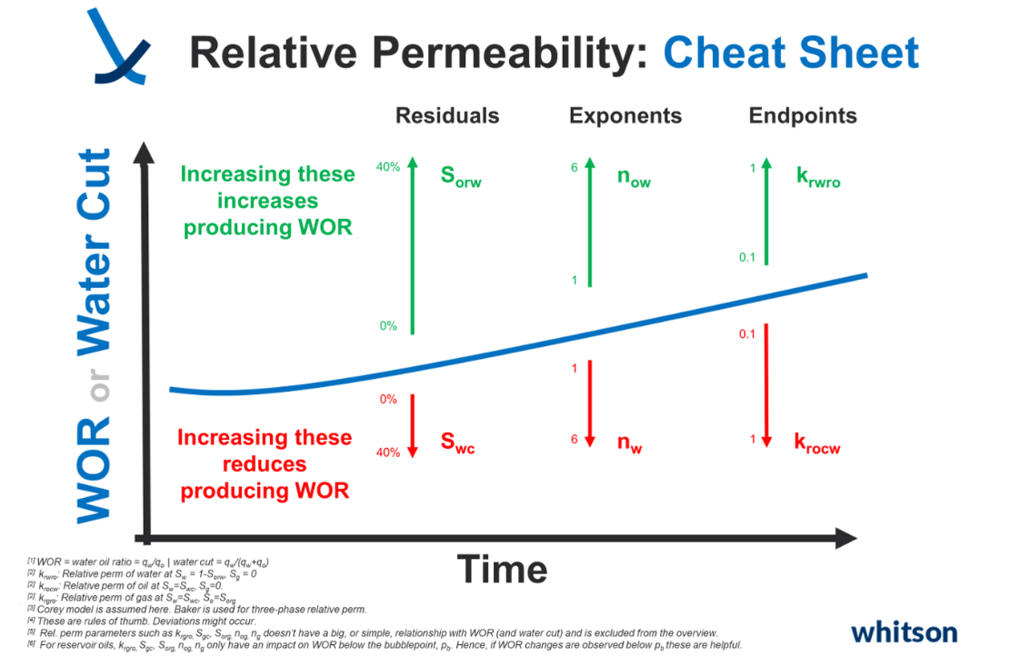
2.1.5 Relative Permeability

1. Open the Relative Permeability Input Card
   • You can adjust the relative permeability parameters to improve the history match.
2. Click SAVE.
3. All steps are shown in the .gif above.

Practical Matching Steps

This workflow outlines the essential steps for practical Numerical RTA calibration (click here).
1. Match Stabilized Water Cuts to ensure the model correctly captures late-time water production behavior.
2. Match GOR Trends to constrain the oil-in-place (OOIP) and fluid behavior.
3. Interpret the Bowie Plot after water cuts and GORs are matched.

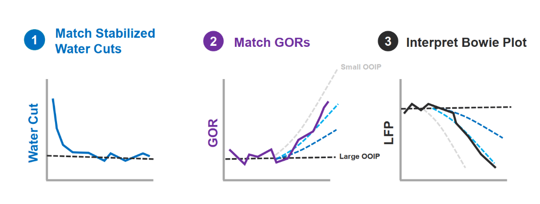
Understanding how relative permeabilities affect Gas-Oil Ratio (GOR) and Water-Oil Ratio (WOR), or water cut, can be tricky. To simplify this, especially for beginners, we've created cheat sheets to help out.

2.1.6 Well Data

1. Click on the EDIT WELL SCHEDULE at the top.
2. In the Numerical Model module, the Well Control is set to BHP (synthetic), as we are using a synthetic well.
   • This means the model is controlled using bottomhole pressure.
   • In this tab, users can also adjust parameters such as minimum BHP, time to reach minimum BHP, simulation start time, and total simulation days.
3. Click RUN to the upper left to run the model.
4. All steps are shown in the .gif above.

2.1.7 Results

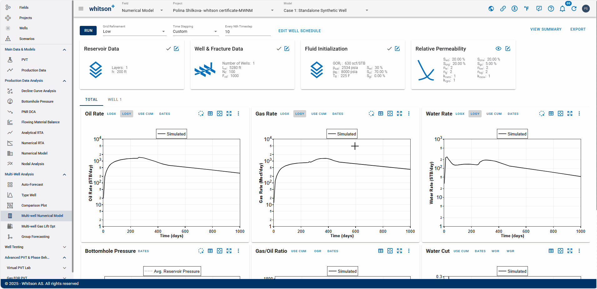
1. At the top right, click VIEW SUMMARY.
   • This tab displays the results table, which includes the following key metrics: Cumulative production (oil, gas, water), OOIP, OGIP, OWIP, and \(A\sqrt{k}\)
2. All steps are shown in the .gif above.

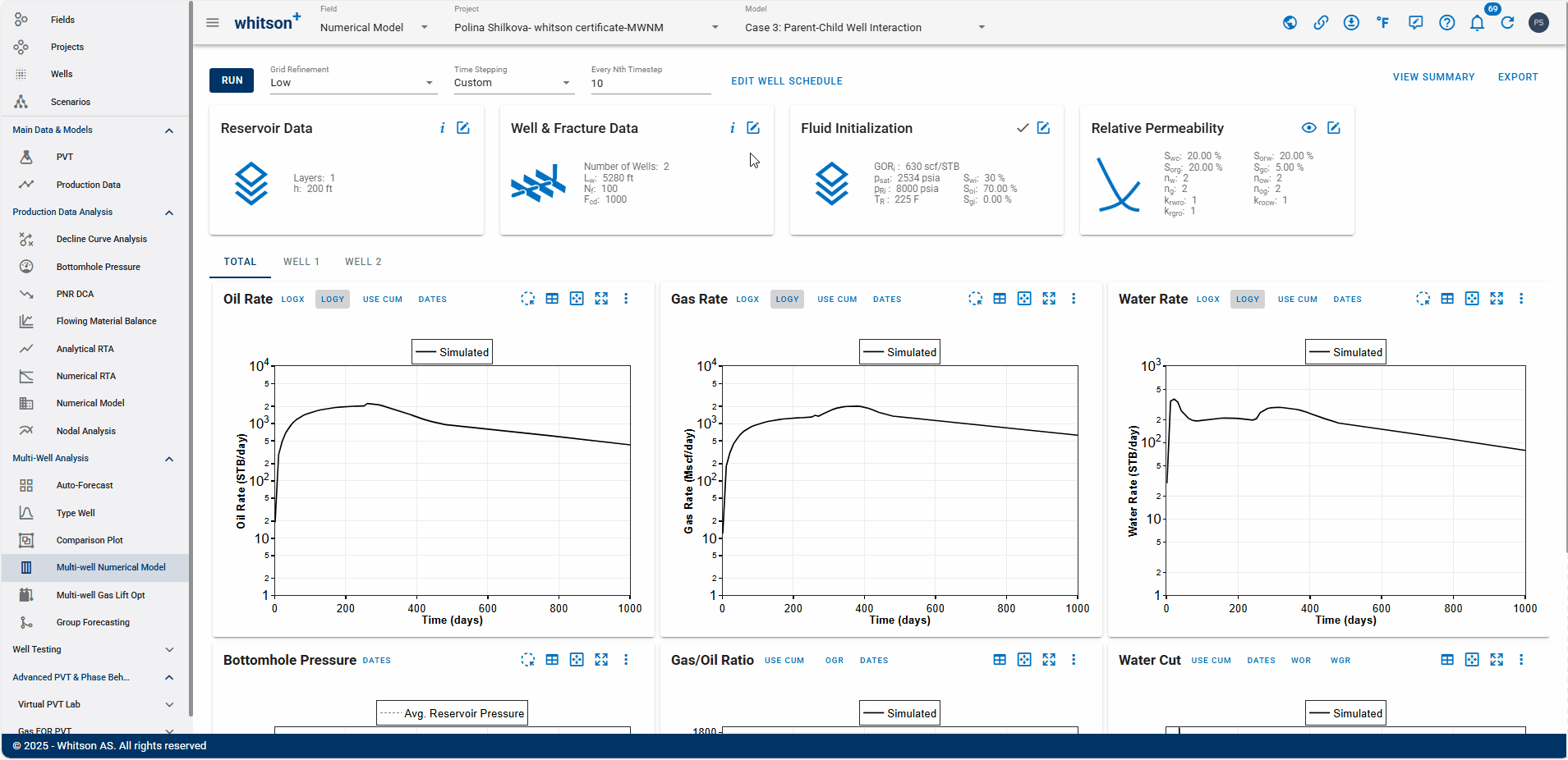
2.2 Case 2: Parent-Child Well Interaction

This case examines the impact of parent–child interactions by modeling three synthetic wells.

2.2.1 Create a Project

1. Go to the Multi-Well Numerical Model module in the navigation panel.
2. Click ADD MULTI-WELL MODEL up to the right.
3. Provide a name and select all the wells by clicking the check box at the top of the well list (left of Well Name).
4. Click ADD MULTI-WELL MODEL.
5. All steps are shown in the .gif above.

2.2.2 Well & Fracture Data

1. Open the Well & Fracture Data Input Card
2. Change the Fracture Halp Length from 400 to 300.
3. Set the Distance to Next Well to 1500 for both wells.
4. Click SAVE.
5. All steps are shown in the .gif above.

2.2.3 Fluid Initialization

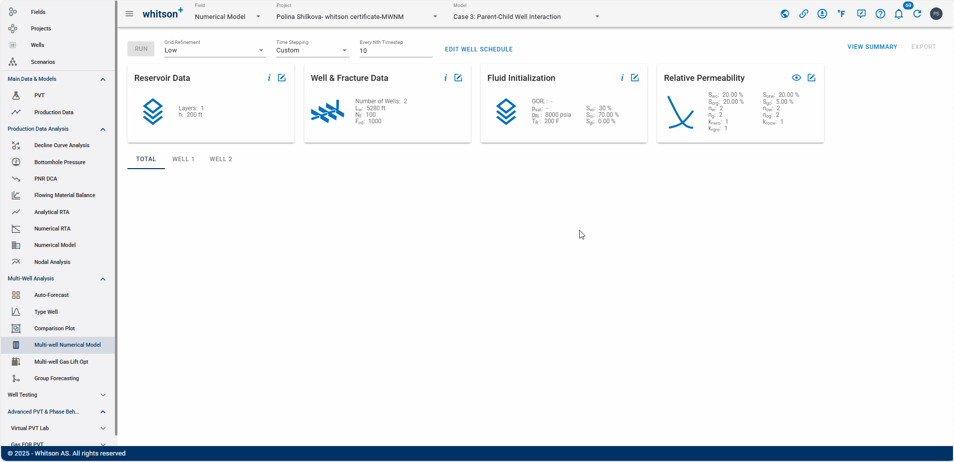
1. Open the Fluid Initialization Input Card
2. Click on PVT from the well and select 5 SWIFT to assign PVT information to the synthetic well.
3. Click SAVE.
4. All steps are shown in the .gif above.

2.2.4 Well Data

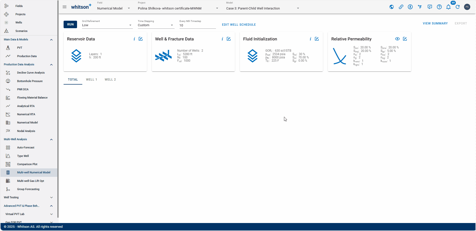
1. Click on the EDIT WELL SCHEDULE at the top.
2. In the Numerical Model module, the Well Control is set to BHP (synthetic), as we are using a synthetic well.
   • Set the simulation duration to 1000 days, matching the previous case to allow for a direct comparison of field development impact.
3. Click RUN to the upper left to run the model.
4. All steps are shown in the .gif above.

2.2.5 Results

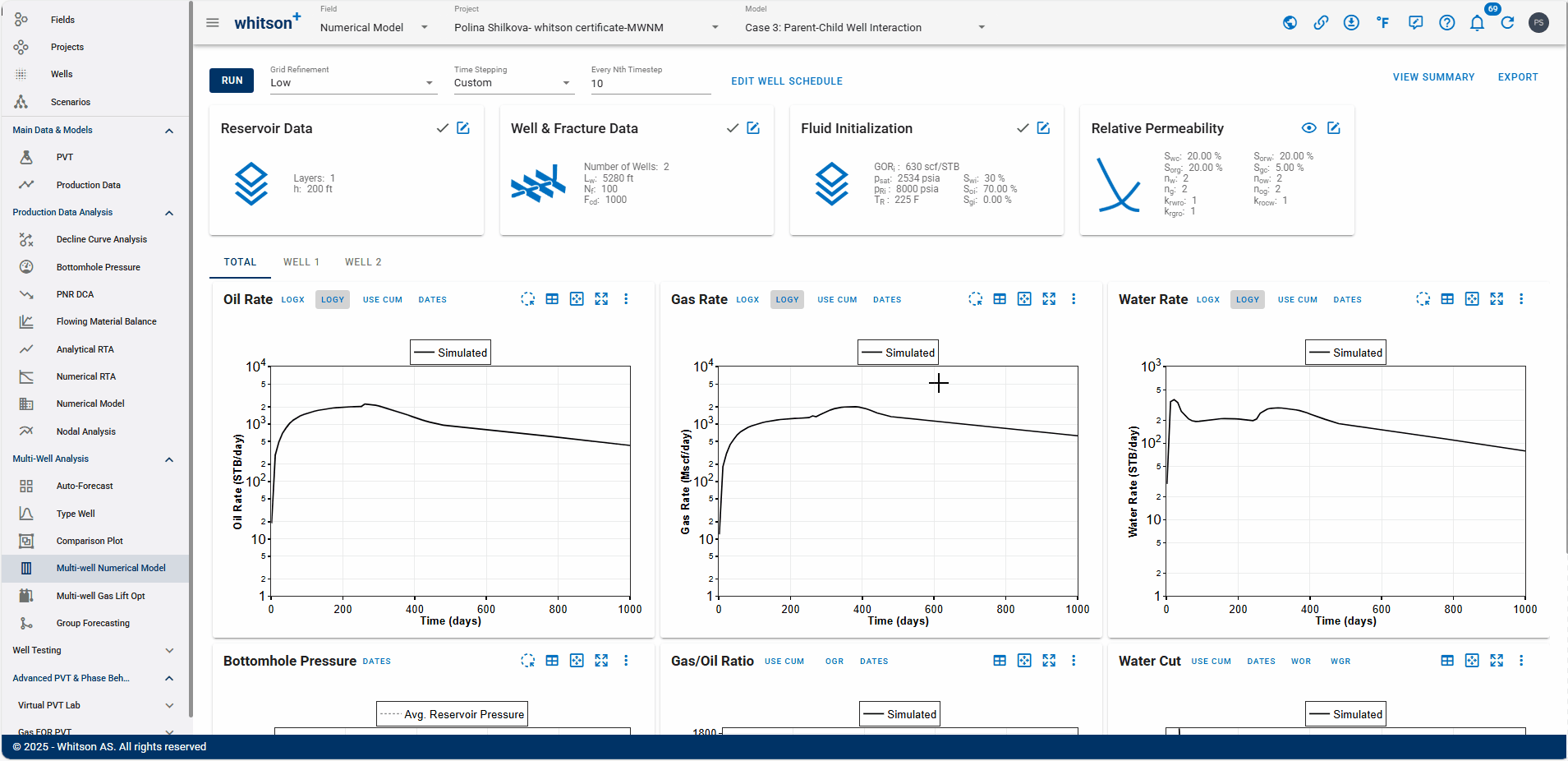
1. At the top right, click VIEW SUMMARY.
2. Compare the results with the previous model.
3. All steps are shown in the .gif above.

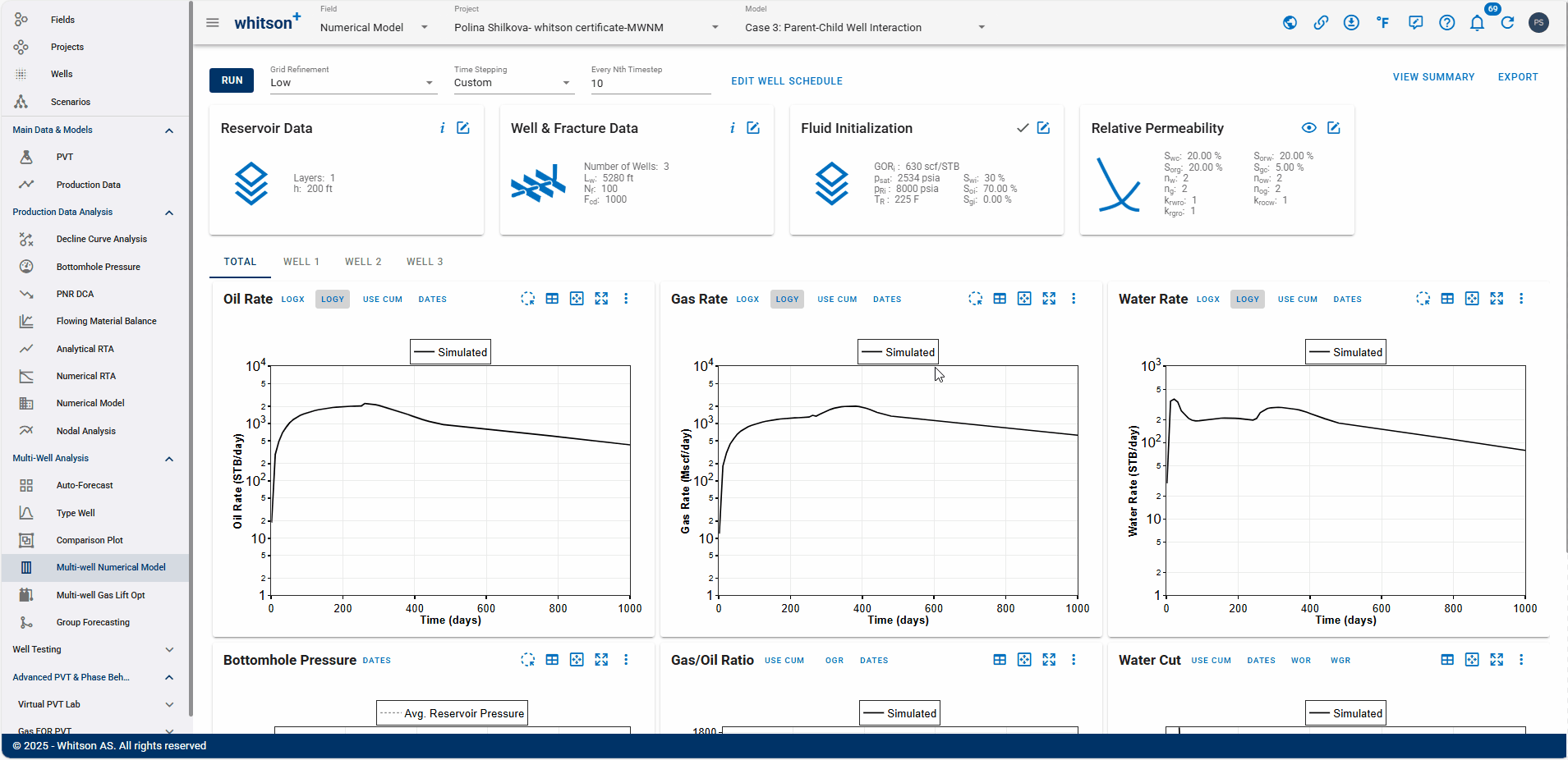
2.2.6 Adding a Child Well

In this scenario, we’ll insert a child well between two existing wells after 450 days of production to evaluate its impact on performance.

1. Open the Well & Fracture Data Input Card
2. Add a new well by clicking the “+” icon in the top right corner.
3. Set the Fracture Halp Length to 300.
4. Change the Distance to Next Well to 750 for all three wells.
5. Click SAVE.
6. All steps are shown in the .gif above.

2.2.7 Well Data

1. Click on the EDIT WELL SCHEDULE at the top.
2. In the Numerical Model module, the Well Control is set to BHP (synthetic), as we are using a synthetic well.
3. For the second (child) well, set:
   • Simulation Start Time to 450
   • Total Simulation Days to 550
4. Click SAVE.
5. Click RUN to the upper left to run the model.
6. All steps are shown in the .gif above.

2.2.8 Results

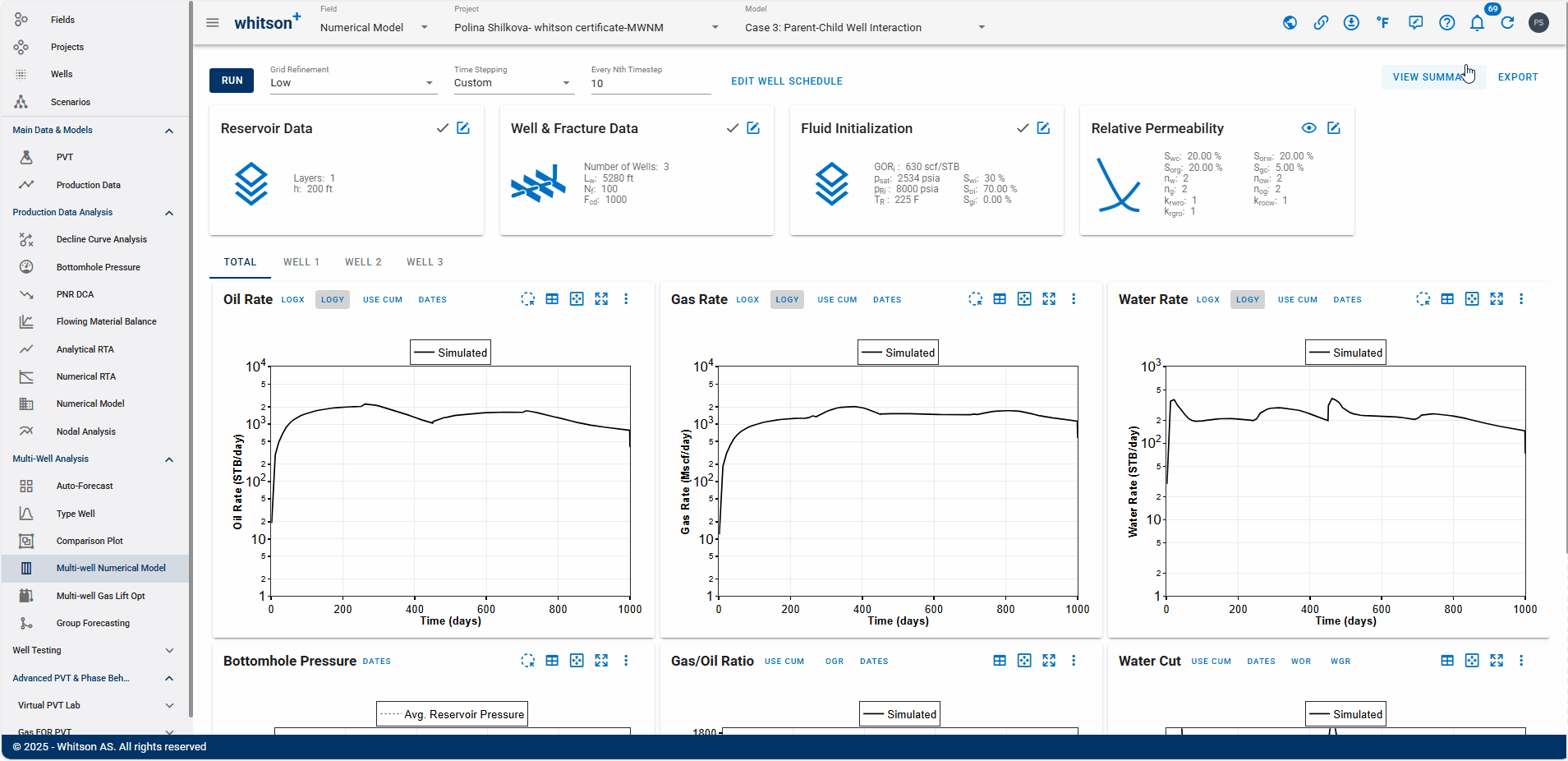
1. At the top right, click VIEW SUMMARY.
2. Compare the results with the previous model.
   • What can you observe about the production effectiveness?
3. All steps are shown in the .gif above.

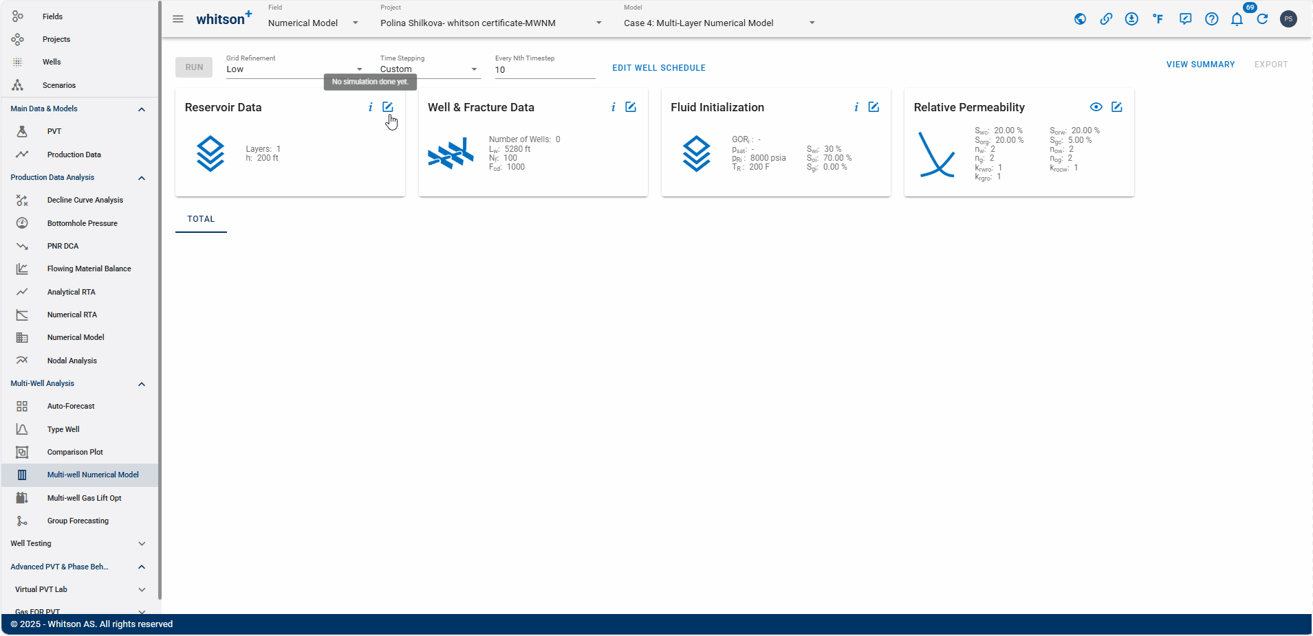
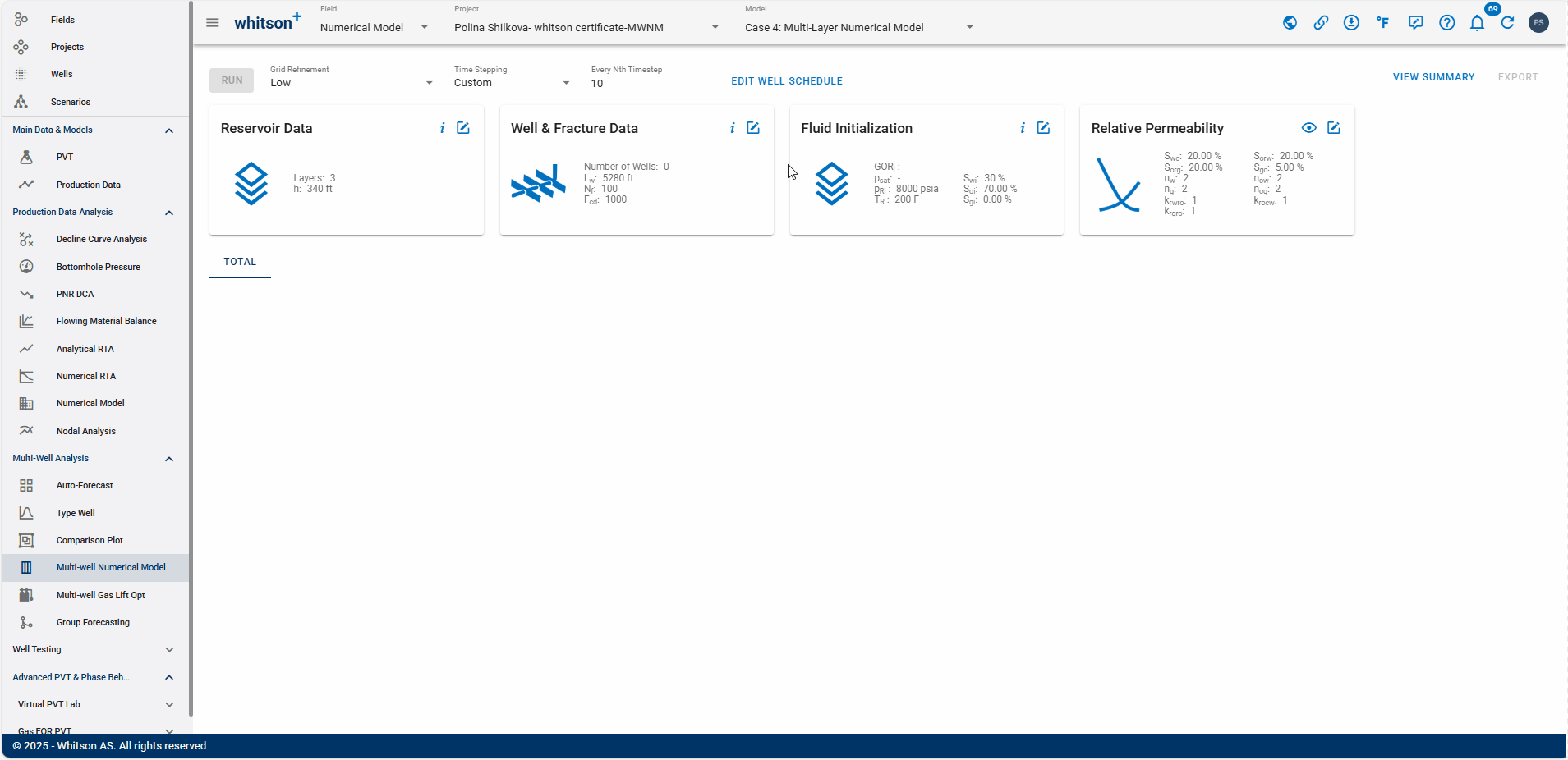
2.3 Case 3: Multi-Layer Numerical Model

We extend the workflow to a more complex multi-layer development using two synthetic wells in one layer combined with a synthetic well in a different layer to represent a stacked development. This setup allows us to study inter-layer interactions and evaluate stacked/offset well strategies.

2.3.1 Create a Project

1. Go to the Multi-Well Numerical Model module in the navigation panel.
2. Click ADD MULTI-WELL MODEL up to the right.
3. Provide a name and select all the wells by clicking the check box at the top of the well list (left of Well Name).
4. Click ADD MULTI-WELL MODEL.
5. All steps are shown in the .gif above.

2.3.2 Reservoir Data

1. Open the Reservoir Data Input Card
2. Add new layers by clicking the “+” icon in the top right corner.

3. Input the following reservoir parameters:

   
   

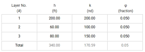
4. Click SAVE.

5. All steps are shown in the .gif above.

2.3.3 Well & Fracture Data

1. Open the Well & Fracture Data Input Card
2. Add a new well by clicking the “+” icon in the top right corner.
3. For Well 2:
   • Select 2 perforated layers.
   • Set Fractured Layers to 1, 2, 3.
4. Set the Fracture Half Length as follows:
   • Wells 1 and 3: 300
   • Well 2: 400
5. Set the Distance to Next Well to 750 for all three wells.
6. Click SAVE.
7. All steps are shown in the .gif above.

2.3.4 Fluid Initialization

1. Open the *Fluid Initialization Input Card.
2. Click on PVT from the well and select 5 SWIFT to assign PVT information to the synthetic well.
3. Click SAVE.
4. All steps are shown in the .gif above.

2.3.5 Results

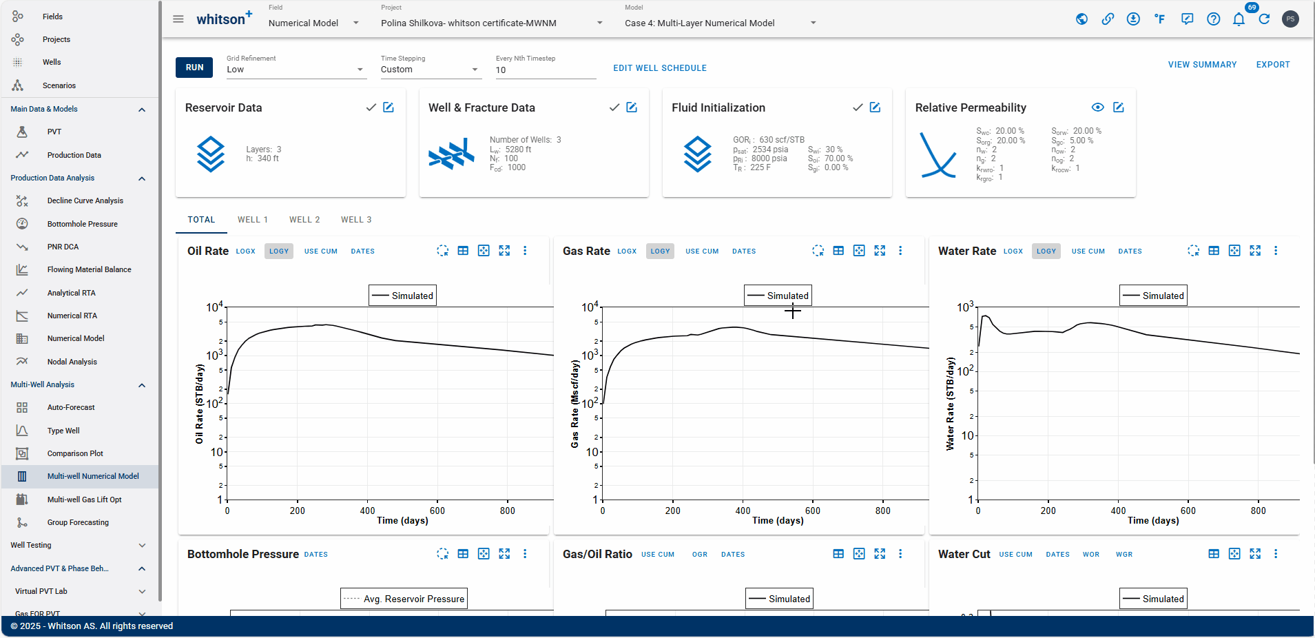
1. At the top right, click VIEW SUMMARY.
2. Compare the results with the previous model.
3. All steps are shown in the .gif above.

Based on the analysis of the three well stacking and spacing scenarios, which field development plan do you consider the most effective, and why?

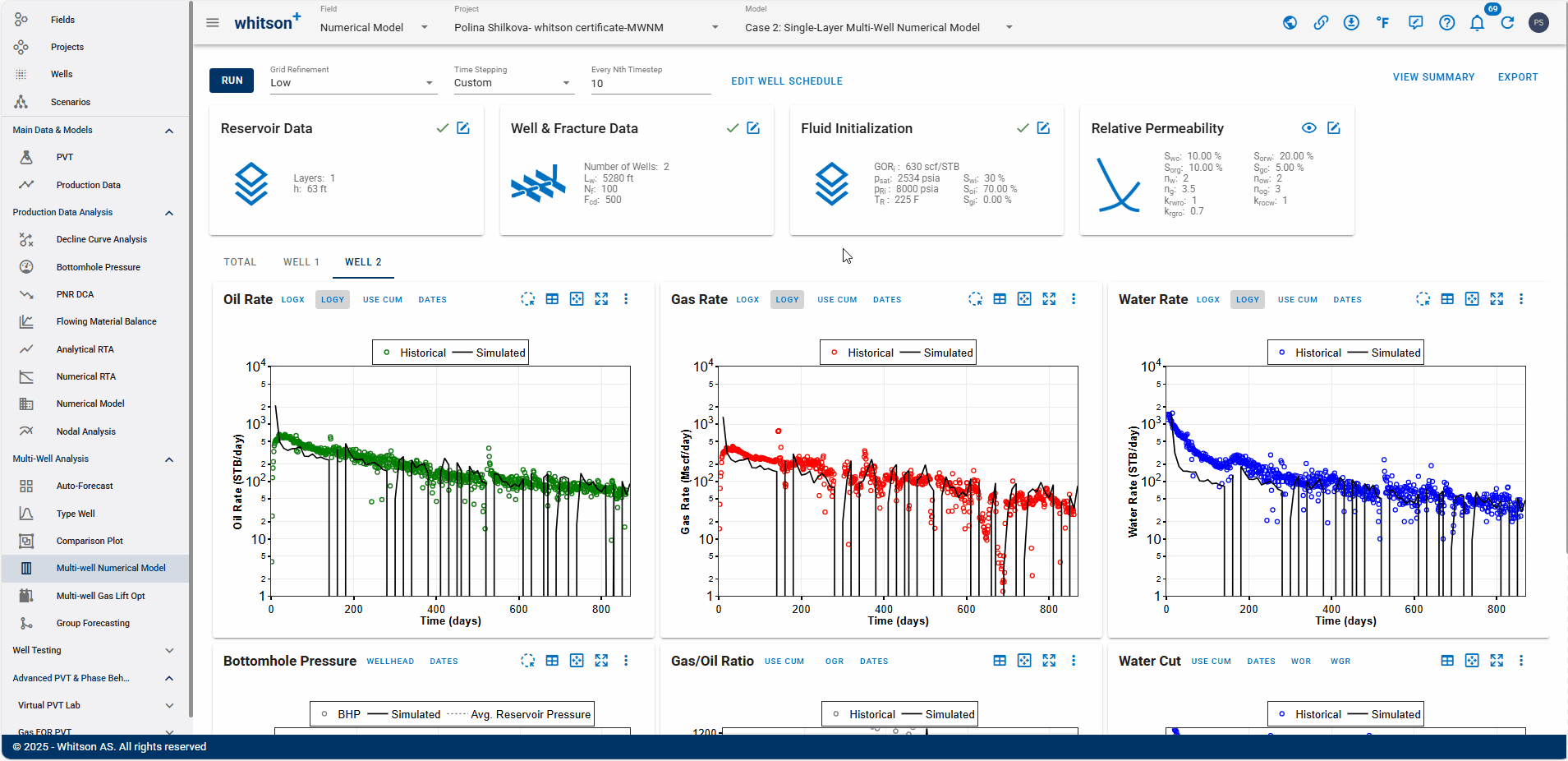
2.4 Case 4: Single-Layer Multi-Well Numerical Model

In this case we move from a standalone well to a single-layer system with multiple wells. In this case, we compare two real standalone wells against the same wells under different completion designs. This allows us to investigate how variations in well spacing and completion strategy influence cumulative recovery, productivity, and reservoir drainage.

2.4.1 Create a Project

1. Go to the Multi-Well Numerical Model module in the navigation panel.
2. Click ADD MULTI-WELL MODEL up to the right.
3. Provide a name and select all the wells by clicking the check box at the top of the well list (left of Well Name).
4. Click ADD MULTI-WELL MODEL.
5. All steps are shown in the .gif above.

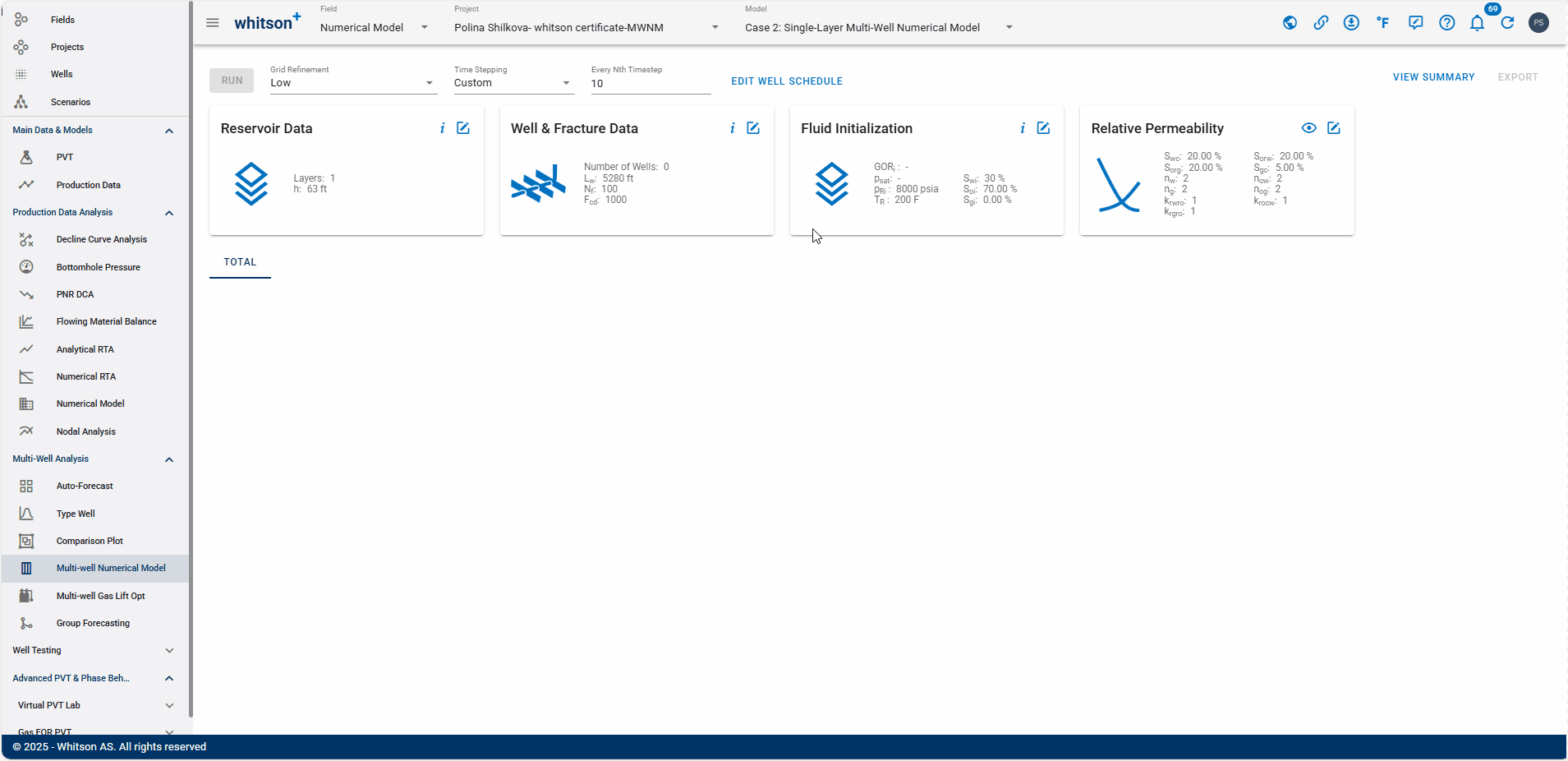
2.4.2 Reservoir Data

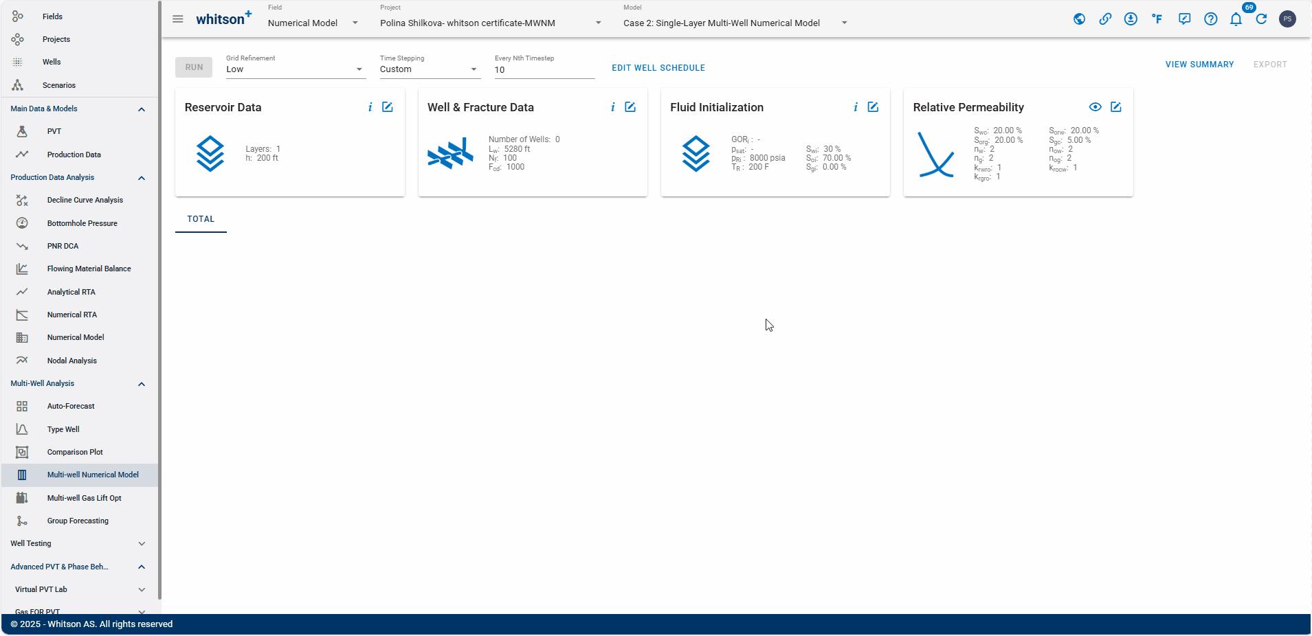
1. Open the Reservoir Data Input Card.
2. Enter the following values:
   • Reservoir Height: 62.8
   • Matrix Permeability: 350
   • Fracture and Matrix Gamma: 2
3. Click SAVE.
4. All steps are shown in the .gif above.

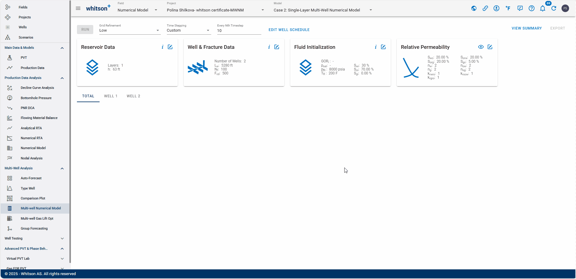
2.4.3 Well & Fracture Data

1. Open the Well & Fracture Data Input Card.
2. Input a Dimensionless Frac Conductivity of 500.
3. Link the first well to WELL-5-SWIFT, and the second to the WELL-6-SPARROW.
4. Click SAVE.
5. All steps are shown in the .gif above.

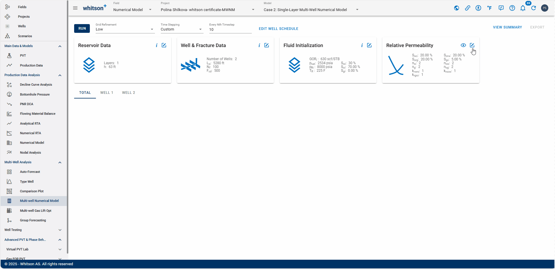
2.4.4 Fluid Initialization

1. Open the Fluid Initialization Input Card.

2. Click on PVT from the well and select 5 SWIFT to assign PVT information to the synthetic well.

3. Click SAVE.

4. All steps are shown in the .gif above.

2.4.5 Relative Permeability

1. Open the Relative Permeability Input Card.
2. Adjust the relative permeabilities
   1. S_wc = 20 -> S_wc = 10 (will increase water cut).
   2. S_org = 20 -> S_org = 10 (will make GOR increase earlier in time).
   3. n_g = 2 -> n_g = 3.5
   4. n_og = 2 -> n_og = 3
   5. k_rgro = 1 -> k_rgro = 0.7
3. All steps are shown in the .gif above.

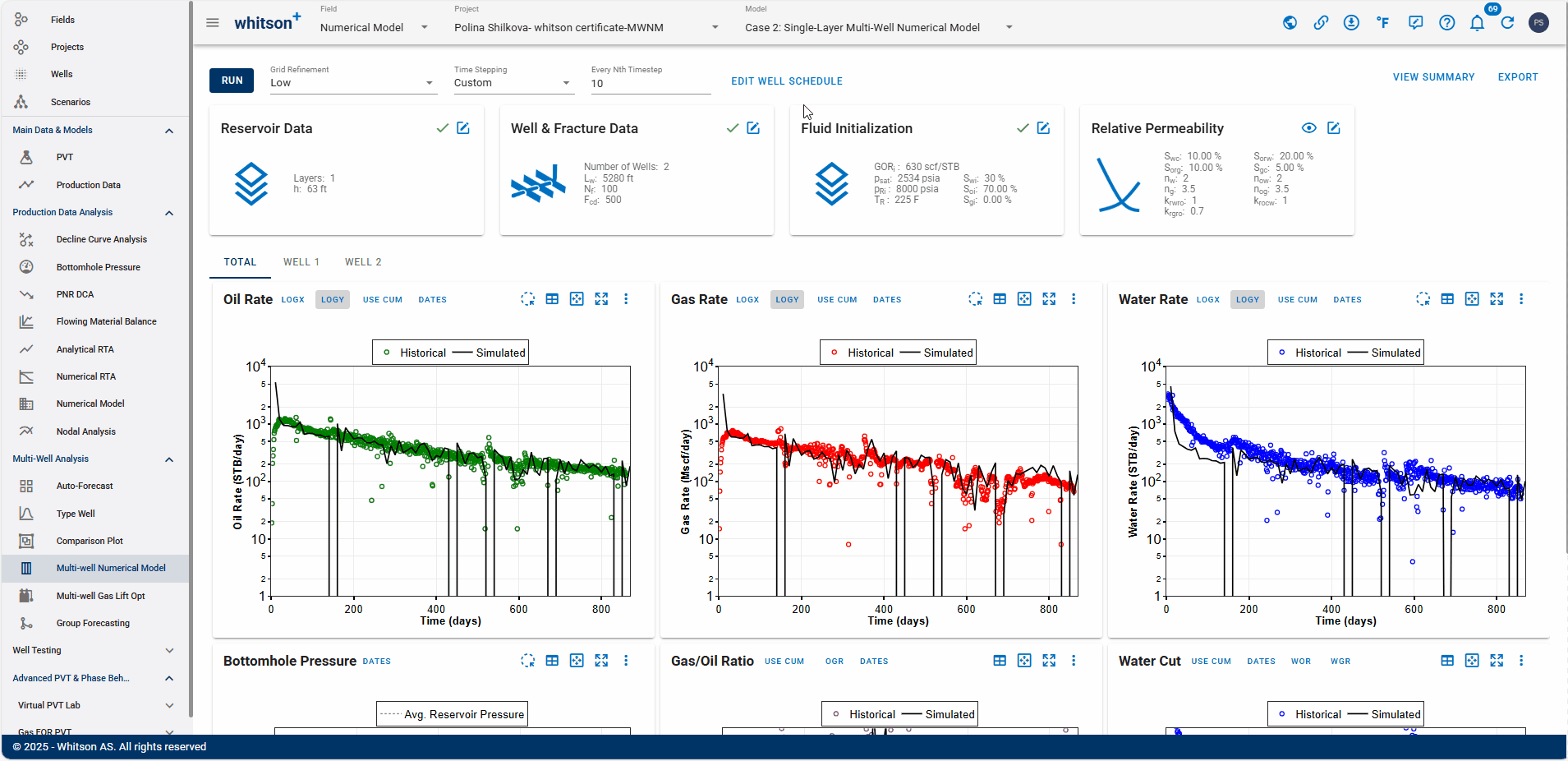
2.4.6 Well Data

1. In the WELL SCHEDULE module, change the Well Control to BHP.
   1. This means we are controlling the model on bottomhole pressure.
2. Click RUN to the upper left, again.
3. This run should also be a very good history match, as none of the parameters have changed, only the well control. And this means:
   1. Your bottomhole pressure should be spot on (as you control the model on BHP).
   2. Your gas rate fit should be great.
   3. Your water rate match could improve (we didn't do much here).
4. All steps are shown in the .gif above.

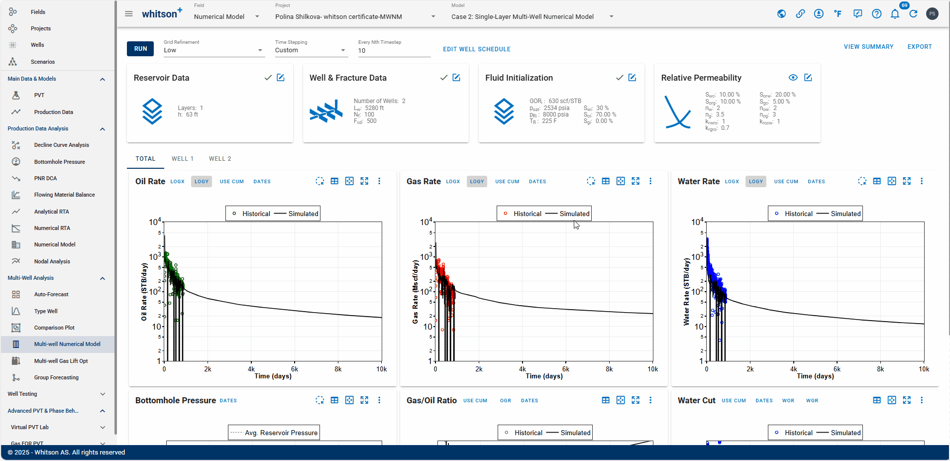
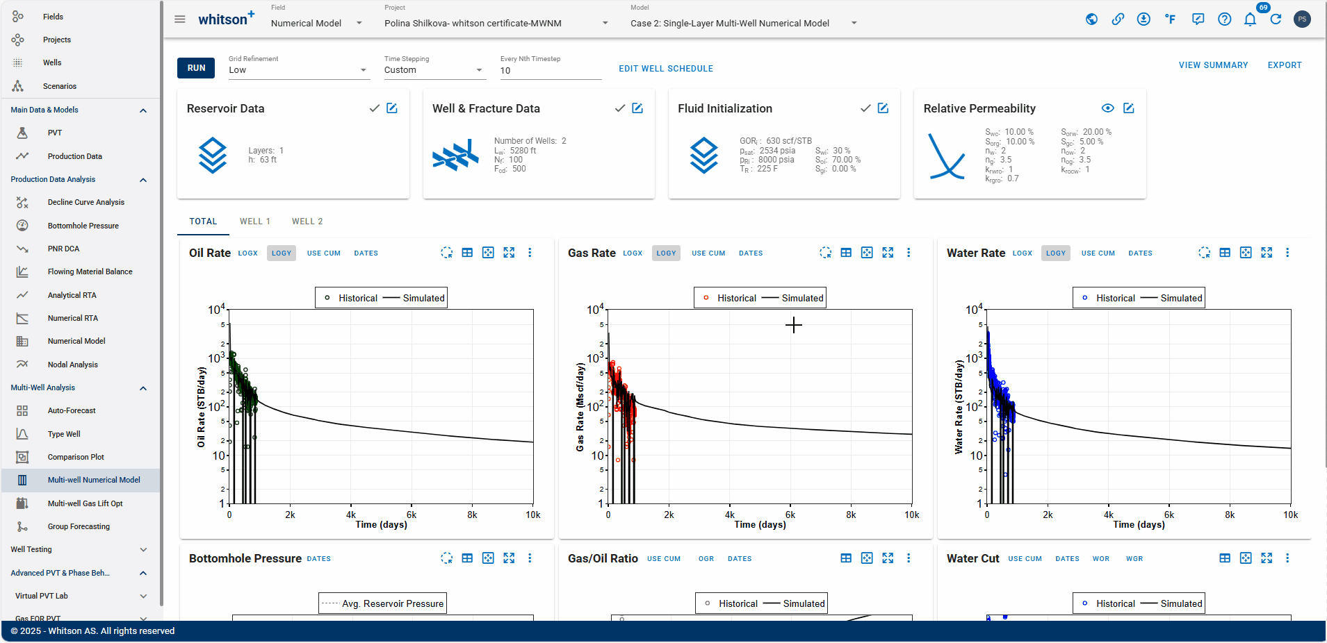
2.4.7 Forecast

1. Click on EDIT WELL SCHEDULE again.
2. Toggle the switch Include Forecast on.
3. Click the text EDIT FORECAST SCHEDULE.
4. Here, you can now forecast the wellhead pressure (WHP) or the bottomhole pressure (BHP)
5. Let's forecast the BHP - The Forecast type is Parametric Decline.
   1. Make the Forecast End Time 10,000 days (almost 30 years).
   2. Make the Forecast Start Day 850.
6. Click SAVE.
7. Click RUN to the upper left, again.

2.4.8 Results

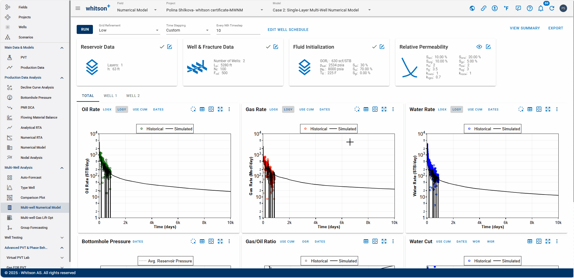
1. At the top right, click VIEW SUMMARY.
   • This tab displays the results table, which includes the following key metrics: Cumulative production (oil, gas, water), OOIP, OGIP, OWIP, and \(A\sqrt{k}\)
2. All steps are shown in the .gif above.

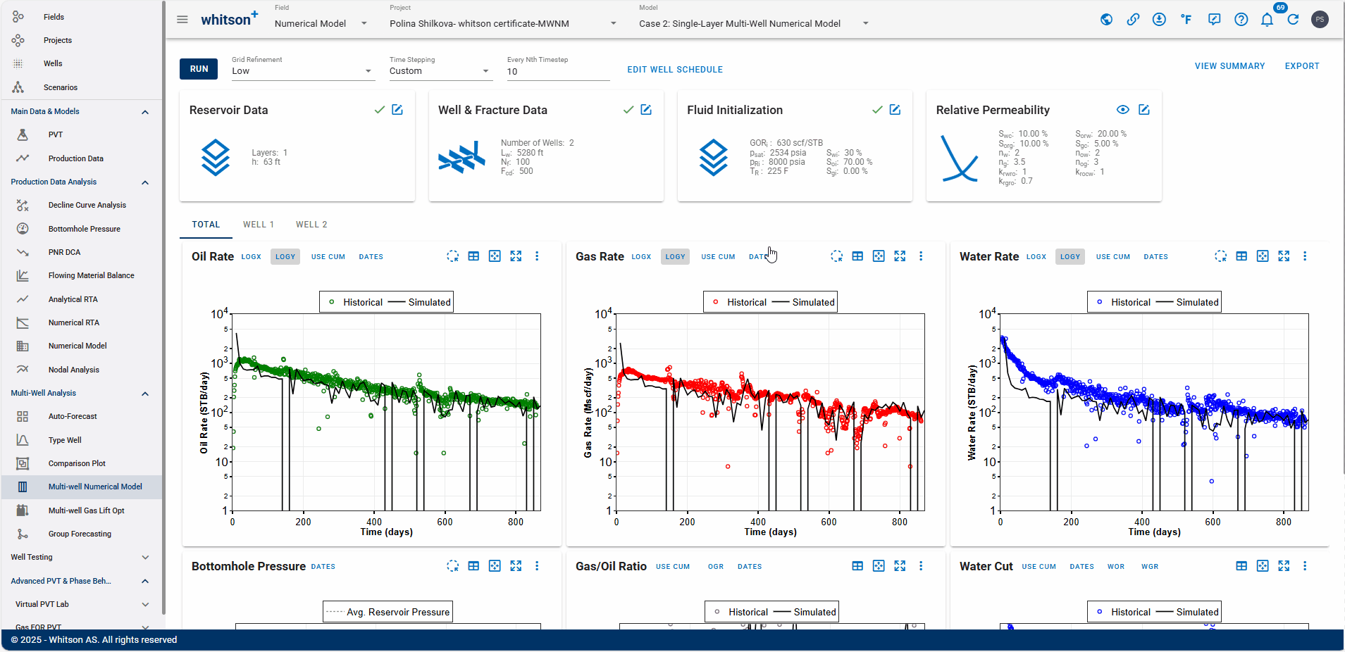
2.4.9 Remove the Forecast

1. Click on EDIT WELL SCHEDULE again.
2. Toggle the switch Include Forecast off. This completely removes the forecast from the plots.
3. Click RUN to the upper left, again.
4. All steps are shown in the .gif above.

2.4.10 Different Completion

Now let's try a case with a different completion.

1. Open the Well & Fracture Data Input Card.
2. Change the Fracture Halp Length from 400 to 500.
3. Click SAVE.
4. All steps are shown in the .gif above.

2.4.11 Forecast

1. Click on EDIT WELL SCHEDULE again.
2. Toggle the switch Include Forecast on.
3. Click the text EDIT FORECAST SCHEDULE.
4. Here, you can now forecast the wellhead pressure (WHP) or the bottomhole pressure (BHP)
5. Let's forecast the BHP - The Forecast type is Parametric Decline.
   1. Make the Forecast End Time 10,000 days (almost 30 years).
   2. Make the Forecast Start Day 850.
6. Click SAVE.
7. Click RUN in the upper-left corner to run the updated model.
8. All steps are shown in the .gif above.

2.4.12 Results

1. At the top right, click VIEW SUMMARY.

2. Compare the results with the previous model.

   • What can you observe about the production effectiveness?
   • Which case appears more optimal for field development planning and optimization?

3. All steps are shown in the .gif above.

3. Done?

When you are done with your Multi-Well Numerical Model certification, please:

1. Send an e-mail to certification@whitson.com
2. Make the subject: "whitson⁺ MWNM certificate: [YOUR NAME HERE]".
3. Include the link to your project.
4. If you have any notes, comments, or observations related to the well, feel free to share them with us. Also, feedback on the user-friendliness of the software is always appreciated.