Pressure Normalized Rate (PNR) DCA
1. Basic Principles
1.1. PNR for Oil
The Pressure-Normalized Rate (PNR) method relates production rate to pressure drawdown. We can calculate the PNR for oil using equation below:
where, is the oil production rate, is the initial reservoir pressure, and is the flowing-bottomhole pressure (BHP).
1.2. PNR for Gas
The PNR method for gas follows the same fundamental principles as for oil but incorporates pseudo-pressure terms to account for the nonlinear changes in gas properties with pressure. This adjustment is essential because gas compressibility and viscosity vary significantly with pressure, making conventional PNR-based calculations less reliable for gas reservoirs. The equation of PNR for gas is as below:
and, represents the pseudo-pressure function, and can be defined as:
where, is the gas viscosity and is the gas compressibility factor.
1.3. PNR Flowrate
Xie (2023) identified that performing DCA in unconventional wells may lead to an overestimated EUR due to early-time production rates exhibiting a prolonged flat trend. A better approach is to use the PNR flowrate, which is obtained by multiplying the PNR by a constant pressure drawdown to ensure a consistent rate unit:
where, represents the PNR flowrate at a constant pressure drawdown and is the minimum or abandonment BHP.
2. Practical Aspects
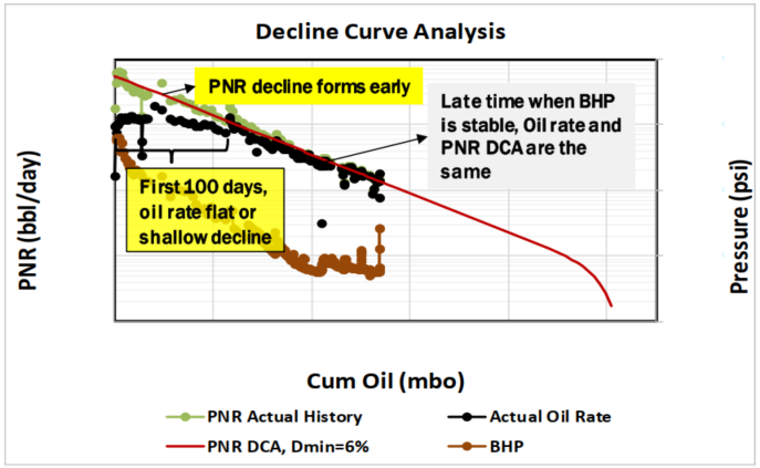
The PNR flowrate decline trend converges to the actual rate decline trend when BHP is considerably stabilize. In the figure below, the late-time trends of PNR flowrate and actual oil rate are converge. This result demonstrates that performing DCA on PNR flowrate is more reliable than using actual rates, which are highly uncertain, especially in early-time data.
Another key advantage of this method is that the PNR flowrate decline trend is formed at early-time, and when we extend the decline trend to the end of historical period, it aligns well with the actual production trend.
Source: Xie, Xueying (2025)
2.1. PNR DCA Methodology
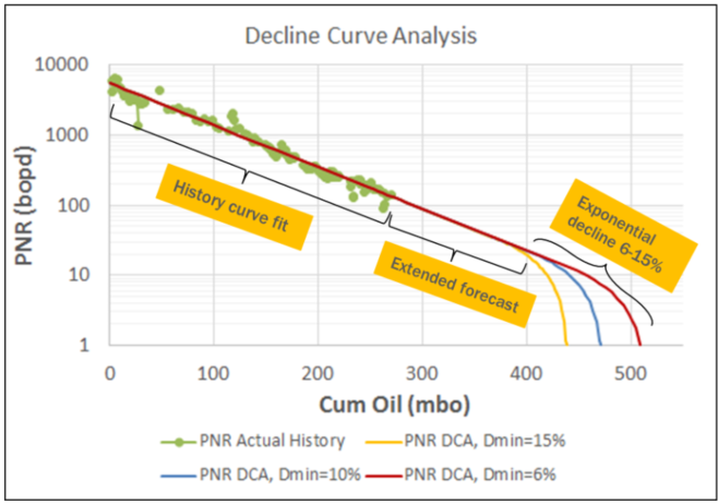
Performing DCA on PNR flowrate provides a more reliable EUR estimation as it integrates both rate and pressure decline,overcoming early-time challenges. The methodology involves:
- Plotting the PNR flowrate vs cumulative production.
- Performing a history match curve fit for the identified decline segment(s).
- Forecasting production using the fitted decline parameters until the end of the well's life.
Source: Xie, Xueying (2025)
2.2. Practial Tips
Here are some practical guidelines for using PNR DCA
- For a starting point, setting = 1 has shown to provide a good fit.
- Be cautious when using data within the first 30 days, as early-time data can be highly influenced by the initial reservoir pressure ().
- The minimum or limiting decline rate ( or ) can be assumed in a range to obtain EUR uncertainty.
3. PNR DCA in whitson+
3.1. Autofit
The autofit algorithm identifies the last 50% data that is non-zero and fits the PNR DCA parameters to this portion. A sequence of zero rates in the data typically indicates a shut-in, requiring re-initialization of the PNR DCA fit.
3.1.1. Residual Function
The fitting routine uses the following residual function in the least squares routine:
where is the residual at time , is the weight factor of time \(i\), is the time index and is the production rate.
3.1.2. Default Bounds
| Parameter | Lower Bound | Higher Bound | Unit |
|---|---|---|---|
| \(q_i\) | 40% of max observed q | 20% higher than max observed q | volume unit / time |
| \(a_i\) | 0 | 10 | / yr |
| \(b\) | 0.5 | 1.2 | - |
3.1.3. Adjusting Default Autofit Bounds on PNR DCA Parameters
You can adjust the autofit settings by modifying the decline parameter ranges for the default modified Arps decline.
- In the modified Arps decline, the function automatically adds a final exponential-decline segment once the minimum or limiting effective decline rate is reached.
- You can also lock specific DCA Segment parameters, forcing that the autofit function calculates using the provided input values.
3.1.4. Weighting factors
By default, all days have a weighting factor of 1, except when = 0, where the weighting factor is set to 0.
3.2. General tips
3.2.1. Manually Adjusting PNR DCA Parameter Graphically
In whitson+, users can manually adjust specific points on the PNR DCA plot, each influencing different parameters that define the production decline trend.
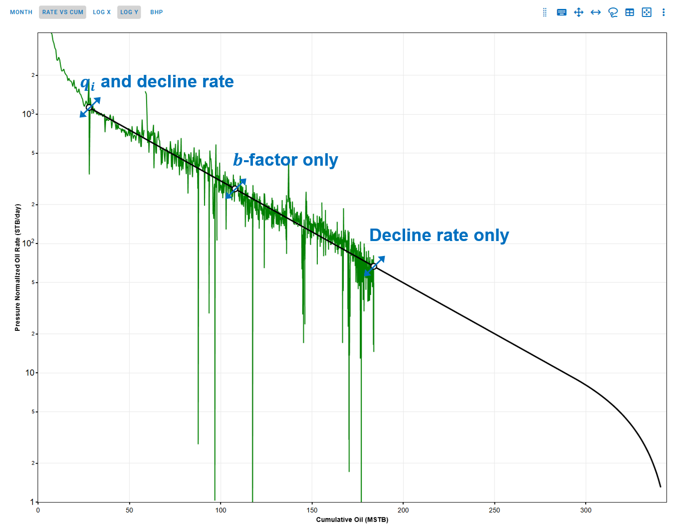
Adjustment points:
- First point: modifies both the and decline rate. This adjustment impacts the early production and the overall scale of the decline curve.
- Second point: adjusts the -factor, which controls the curvature of the decline trend. A higher -factor leads to a slower decline in production, while a lower -factor results in a steeper drop.
- Third point: alters only the decline rate, influencing the rate at which production decreases over time.
Why manual adjustments matter?
Manually refining these parameters allows users to create more accurate production forecasts, particularly in unconventional reservoirs where decline trends may not fit standard analytical models perfectly. This flexibility helps in optimizing well performance analysis and forecasting long-term production more effectively.
3.2.2. Rate-Cum Decline vs Rate-Time Decline
You can view the decline fit in:
- Rate vs. cumulative production plot (default)
- Rate vs. time plot
3.2.3. Converting from Rate-Cum to Rate-Time
When transitioning betweem rate-cum and rate-time domains in DCA, it is essential to perserve consistency, particulartly with Estimated Ultimate Recovery (EUR). However, the relationship between rate, time, and cumulative production are nonlinear and sensitive to segment definition.
To maintain the same EUR in both spaces, whitson+ performs a back calculation of the initial segment parameters when switching between domains.
Rate-Cum:
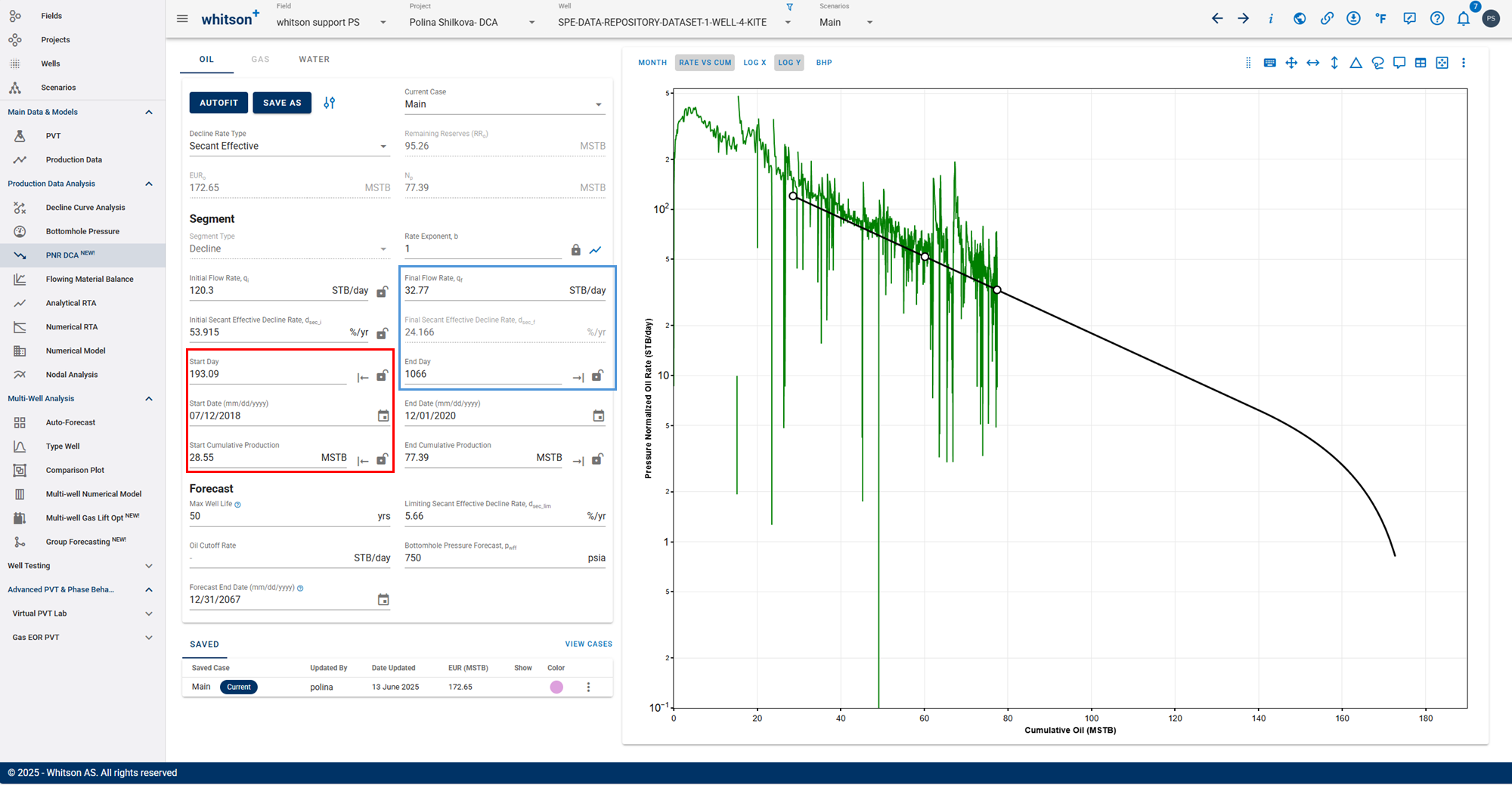
Rate-Time:
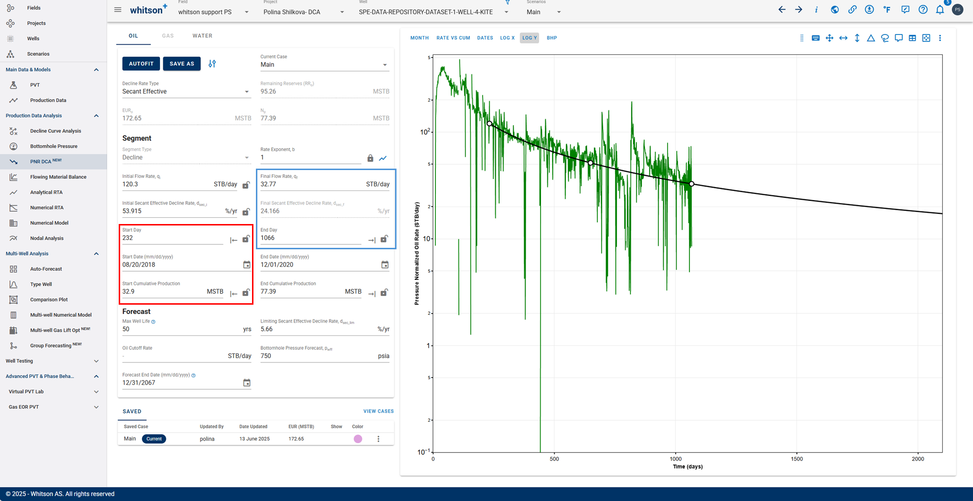
- The forecast end parameters (marked in blue) remain fixed.
- The segment start parameters (marked in red) are recalculated when switching between domains to ensure that cumulative production and EUR remain consistent.
This approach ensures that the cumulative production curve integrates correctly over time, regardless of whether the input is in rate-time or rate-cum space.
Practical Implication
Switching between rate-time and rate-cum in the PNR DCA module automatically recalculates the segment start or end parameters depending on which domain is active, while holding EUR constant.
This ensures:
1. EUR stability between views
2. Accurate forecast matching
3. Avoidance of manual tuning when switching domains
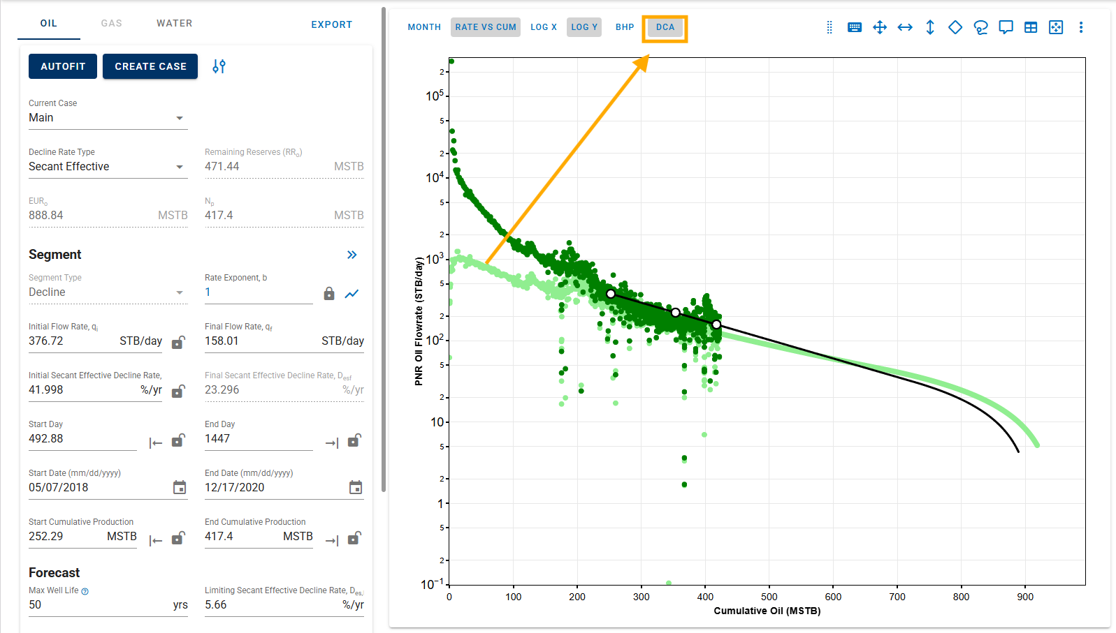
3.2.4. Enable Current DCA Case Visualization within PNR-DCA
You can add an option in PNR-DCA to display the Current Case from the traditional DCA module, enabling easier comparison and improved visualization between the two workflows.
3.2.5. Saving the PNR DCA fit
You can save the current PNR DCA fit as a saved case by using the SAVE CASE button. This allows you to adjust the fit as needed while keeping a checkpoint to revert to if necessary.
- To overlay saved cases in the plot, check the box under the "Show" column for each saved case.
- To reload PNR DCA parameters (and the corresponding fit), use the "Load Case" option available for each saved case by clicking the three vertical dots.
- If a saved case name already exists, you will be prompted to confirm whether to overwrite the existing case to prevent duplicates.
3.3. Using Fractional RTA to Fit PNR DCA
In whitson+, users can initialize PNR DCA parameters using insights from Fractional RTA. This constrains the decline curve analysis by incorporating the time to end of characteristic flow \(t_{ecf}\).
This feature can be used as demonstrated in the GIF below:
3.3.1. Estimate \(\delta\) from Fractional RTA Diagnostic Plots
To begin, we estimate the -parameter, by analyzing the rate normalized pressure (RNP) versus time, , on a log-log scale, followed by a best fit of the power-law function.
Taking logarithms of both sides simplifies the relationship to a straight-line form on a log-log plot, hence, the \(\delta\)-parameter is determined from the slope of the RNP plot.
3.3.2. Use \(\delta\) to Derive the Arps Rate Exponent
There is a relationship between the \(\delta\)-parameter and Arps' -factor. Specifically:
Once \(\delta\) is determined from the slope, the corresponding is used for decline curve modeling.
3.3.3. Fitting PNR DCA Using Fractional RTA Outputs
The Fractional RTA provides:
- \(b\) : Rate Exponent (from \(\delta\))
- \(q_i\) : Flow Rate at \(t_{ecf}\)
- \(t_{ecf}\) : Time to End of Characteristic Flow - used as the Segment Start Day for PNR DCA
With these inputs, the PNR DCA is fitted by performing a linear regression on the Arps equation, using the known \(q_i\), \(b\), and \(t_{ecf}\) values to solve for initial decline rate \(a_i\).
Where:
-
\(q(t)\) is the production rate at time \(t\)
-
\(q_i\) is the rate at \(t_{ecf}\)
-
\(a_i\) is the initial effective decline rate (fitted)
-
\(b\) is the rate exponent from
-
\(t_{ecf}\) is the segment start day
The algorithm:
-
Identifies the last 50% of non-zero production data, avoiding early transient effects
-
Re-initializes fitting if extended zero-rate periods (shut-ins) are detected
-
Using goal-seek to solve for the initial effective decline rate, \(a_i\). This enhancement utilizes a weighted least-squares approach to minimize residuals, improving segment fit accuracy and alignment with the observed data.
where is the residual at time , is the weight factor of time \(i\), is the time index and is the production rate.
3.4. PNR DCA Error Calculations
whitson+ facilitates regression on parameters to minimize the sum of squares of weighted residuals in the context of observed data and corresponding predictions. The objective function is defined as:
Here, represents the RMS residual error between observed measurement and its corresponding prediction, while is the user-assigned weighting factor for that residual. Ideally, these weighting factors should be inversely proportional to the standard deviations of the residuals. Minimizing in provides the maximum likelihood estimation of the model parameters, assuming independent and normally distributed residuals.
The default weighting factors are 1. Reported is a root-mean-square (RMS) residual error () defined as:
This metric is related to but is more easily interpreted.
The residuals are calculated as relative percentages using the formula:
where is the historical production value, is the DCA value, and is the reference value for observation .
For more details on error calculation please refer to the error section in DCA here.
3.5. Hotkeys
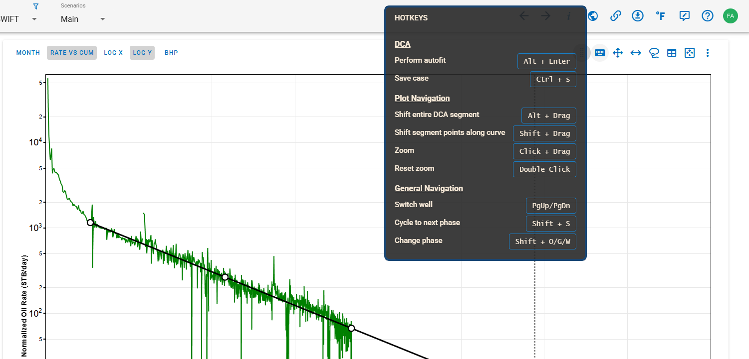
The following hotkeys help streamline workflow and enhance navigation within the software:
3.5.1. Decline Curve Analysis (DCA)
- Perform Autofit: Press
Alt + Enterto automatically fit the decline curve to the available data. - Save Case: Use
Ctrl + Sto save the current case, ensuring no changes are lost.
3.5.2. Plot Navigation
- Shift entire DCA segment: Hold
Altand drag the mouse to shift the entire decline curve analysis segment on the graph. - Shift segment points along curve: Hold
Shiftand drag the mouse to shift the segment points along the curve. - Adjust shape of decline curve: Hold
Ctrland drag the mouse to adjust the shape of the decline curve. - Zoom: Click and drag the mouse over a region to zoom in for a more detailed analysis.
- Reset zoom: Double-click anywhere on the plot to reset the zoom to its default view.
3.5.3. General Navigation
- Switch Well: Use
PgUp/PgDnto navigate between wells in the dataset. - Cycle to Next Phase: Press
Shift + Sto switch between different production phases. - Change Phase: Use
Shift + O/G/Wto toggle between oil, gas, and water phases.