DQI - Devon Quantification of Interference
1. What is DQI?
The Devon Quantification of Interference (DQI) procedure interprets an interference test to estimate the hydraulic diffusivity and the fracture conductivity between the wells. A dimensionless drainage length parameter (LD) is calculated using the conductivity estimate and knowledge of reservoir parameters. The Degree of Production Interference (DPI) is then estimated from the calculated LD. This new metric was defined to quantify the effect of well-to-well interference on production.
For purposes of defining this metric, it was consider a specific case where only two wells have been producing for at least several months. These two wells are bounded by each other on one side, and unbounded on the other side. Then, one of the wells is shut-in, and the objective is to measure the impact on the production rate of the well that remains on production.
2. Procedure - from Almasoodi, Andrews, Johnston and McClure, 2023
2.1. Step 1: Creating Δp and Bourdet derivative plots
Figure 1 shows pressure observations at a monitoring well in a field example in the Meramec formation located in the Anadarko basin of Oklahoma. The vertical black line shows the time when the offset well was put on production, which caused a downward pressure response in the monitoring well.
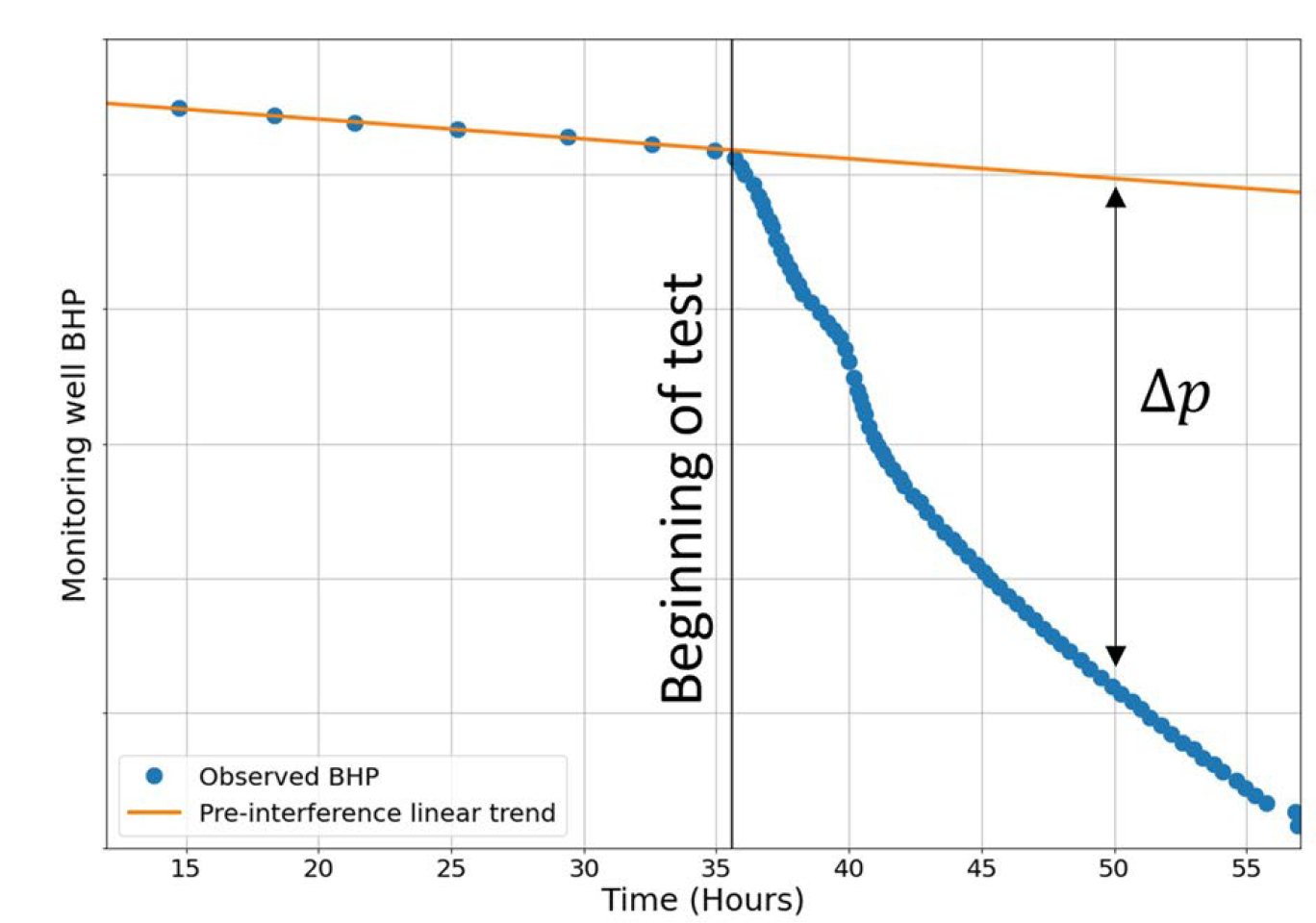
Fig. 1: Pressure observations in a monitoring well before and after the offset well is put on production.
To perform an interpretation, start by constructing a log–log pressure derivative plot showing \(Δp\) and \(t dp/dt\) versus time from the beginning of the transient (Fig. 2). The value \(Δp\) is defined as: \(Δp\) = \(p\) − \(pref\). Where '\(p\)' is the pressure recorded by the pressure gauge, and '\(pref\)' is the extrapolation of the prior pressure decline trend (the orange line in Fig. 1). It may be useful to smooth the data by resampling at increments of pressure.
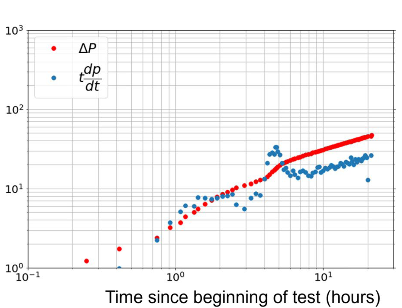
Fig. 2: \(Δp\) and \(t dp/dt\) observed during the interference test.
Figure 3. \(Δp\) and \(t dp/dt\) from the analytical solution (black and blue lines) are fitted to the pressure and derivative observations by a trial and error approach varying \(\alpha\) and \(k\), to find a good fit.
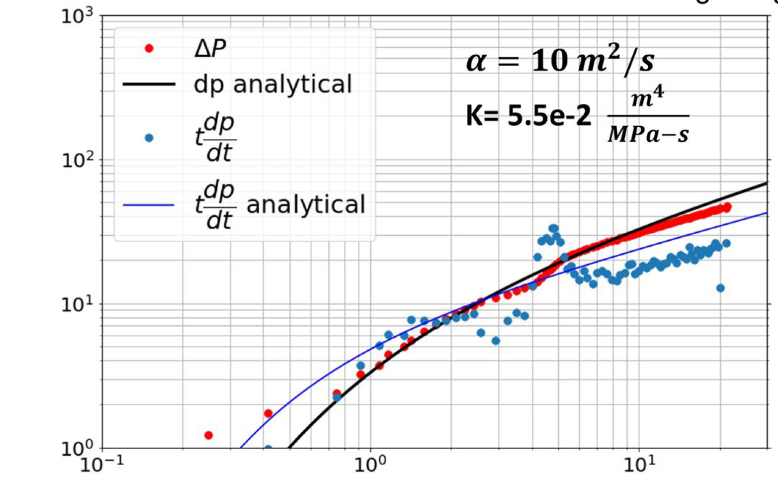
Fig. 3: \(Δp\) and \(t dp/dt\) observed during the interference test.
2.2. Step 2: Computing diffusivity from pressure changes in interference
When the active well is put-on-production, a pressure disturbance propagates along the fracture, as described by the pressure diffusion equation (Zimmerman 2018). In classical well test analysis, the radius of investigation, \(r_{inv}\), is defined as the distance from the well where a pressure disturbance will be felt, as a function of time, \(t\), and hydraulic diffusivity, \(\alpha\) (Horne 1995):
For flow through porous media, the hydraulic diffusivity is equal to the square root of permeability divided by porosity, total compressibility, and viscosity. In a fracture, it is more appropriate to define hydraulic diffusivity in terms of the fracture conductivity and aperture:
Where \(k_f\) is the fracture permeability, \(W\) is the aperture, \(C\) is the fracture conductivity, \(\mu\) is fluid viscosity, \(dW/dp\) is the derivative of aperture with respect to pressure, and \(c_f\) is the compressibility of the fluid in the fracture.
If it is assumed that the fracture is fixed-height, and that the pressure disturbance propagates along the fracture through linear flow, it can be calculated the pressure change from the solution for a constant flux source in a semi-infinite slab (Hetnarski et al. 2014), with the pressure disturbance observed at an offset distance \(y\).
where \(q_0\) is production rate (\(m^3/s\)), \(y\) is offset distance \(m\), \(\alpha\) is diffusivity (\(m^2/s\)), \(K\) equal to , where \(C\) is fracture conductivity, \(H\) is the fracture height, \(\mu\) is the viscosity of the fluid inside the fracture (\(m^4/MPa*s\)).
When plotting the analytical solution, it is observed that the timing of the onset of the pressure interference is controlled by the diffusivity, and the shape of the curve after the onset of interference is controlled primarily by the \(K\) parameter.
It is possible to fit measured data with Eq. 3 and estimate both diffusivity and the \(K\) parameter. However, the estimate of \(K\) is considerably more uncertain than the estimate of diffusivity. It could be affected by: (a) non-constant production rate at the active well, (b) complex fracture geometries other than linear geometry, and (c) change in flow regime from fracture linear (for example, if flow from the matrix causes bilinear flow). Also, nonlinearities could be present during early-time production that—strictly speaking—may violate the linearized ‘single phase’ assumptions that justify: (a) the use a simple diffusivity equation solution (Eq. 3), and (b) the calculation of \(Δp\) = \(p\) − \(pref\) that subtracts out the prior pressure trend (which relies on superposition).
On the other hand, the estimate of diffusivity (from the timing of the onset of the signal) is quite robust. As shown in Eq. 1, the radius of investigation scales with the square root of the product diffusivity and time, regardless of flow regime, flow geometry, or variable boundary condition at the active well. Also, the early-time pressure response of the interference test involves relatively small pressure changes, minimizing the potential impact of nonlinearities in the system, such as changing fluid compressibility.
Thus, the early interference pressure response—the tip of the spear—is the most robust part of the transient for estimating the diffusivity. It is least affected by uncertainties and nonlinearities.
To estimate diffusivity, it was used a trial-and-error approach to fit Eq. 3 to the observed \(Δp\) and \(Δp'\) curves. The value of \(K\) from the curve fit is not used in the rest of the analysis, but it is nonetheless useful to include in the curve fit that it is used for the estimation of the diffusivity. The priority is to fit the part of the trend that matches the initial response—the first 10 s or 100 s of psi. The analytical solution is not expected to be able to match the transient after the initial response. Figure 3 shows an example of fitting the analytical solution to a real interference test. Figure 4 shows sensitivities on the effect of changing the hydraulic diffusivity and \(K\).
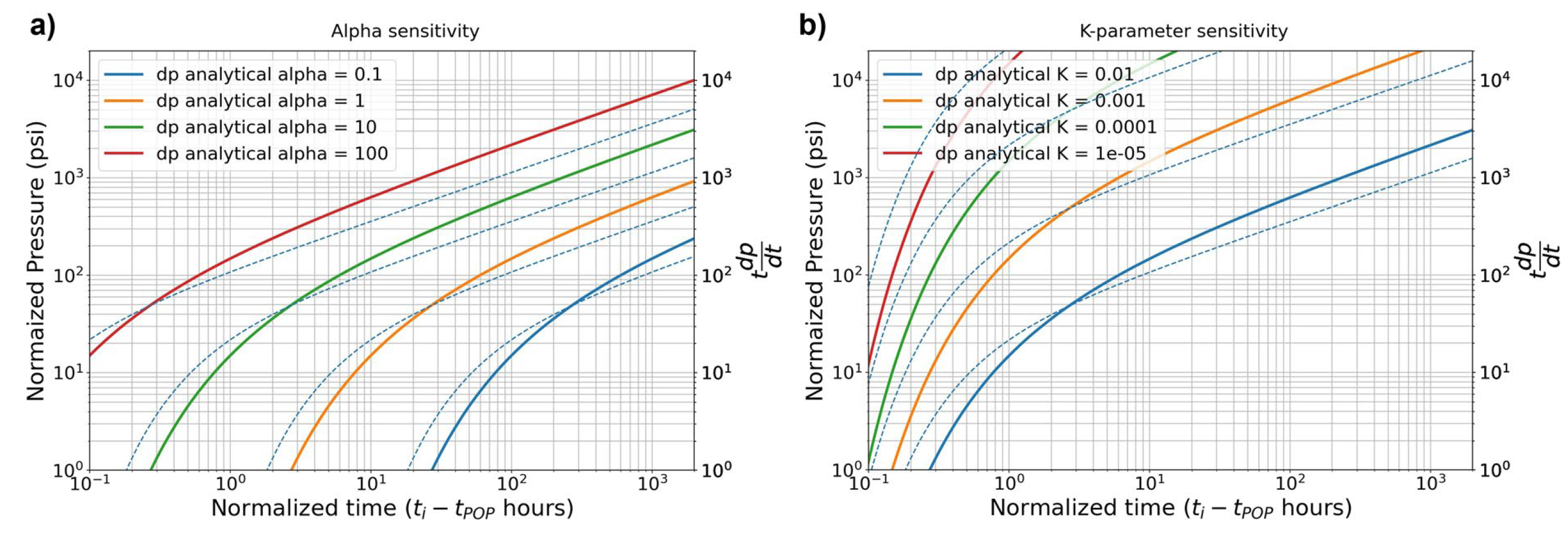
Fig. 4: The variation in \(dp\) (solid lines) and \(t dp/dt\) (dashed lines) at the offset Monitoring Well calculated with the analytical solution with different values of a) \(\alpha\) (keeping \(K\) constant = 0.01), and b) \(K\)-parameter (keeping \(\alpha\) constant = 10). The units of \(\alpha\) are (\(m^2/s\)) and the units of the \(K\)-parameter are (\(m^4/MPa*s\)).
2.3. Step 3: Computing conductivity from diffusivity
Once the diffusivity has been estimated from the curve fit, it can be plugged into Eq. 2 to estimate the fracture conductivity. It will not practically have precise knowledge of \(dW/dp\) and \(W\), but it can plug-in reasonable values:
and \(W\) = 0.76 mm (0.03 in). For \(cf\), it was used the compressibility of the interfering fluid present in the fracture. For the initial POP test after stimulation, this will be the compressibility of water, ∼ 0.000435 MPa−1. For tests performed after months of production, the fluid in the fracture will be a multiphase mixture of oil, gas, and/or water. In this case, it is necessary to use the total compressibility of all the phases in the fracture.
For viscosity, it was used the viscosity of the fluid in the fracture. The initial POP test may be controlled by the viscosity of the frac fluid. For instance, when a viscous HVFR is used for hydraulic fracturing, the POP test viscosity may be influenced by the viscosity of the HVFR which can be significantly higher than water. During the later production phase tests, the effective viscosity of the multiphase mixture must be estimated.
2.4. Step 4: Calculating the dimensionless well spacing
Next, it was necessary to calculate a dimensionless number, \(LD\), that can be roughly defined as the ‘dimensionless drainage distance’. \(LD\) is derived by first approximating \(L\), the ‘maximum possible drainage distance along the fracture if hypothetically it was unbounded and had infinite propped length’. This drainage distance is determined by a balance of flow rate into the fracture and flow rate along the fracture.
The derivation of \(LD\) uses rough ‘back of the envelope’ approximations, but this is acceptable because the objective is not to derive a rigorous analytical solution. Instead, it seeks to determine an appropriate scaling between variables.
To estimate the flow rate along the fracture (towards the well), the Darcy’s law:
where \(Q\), flow rate (\(m^3/s\)); \(H\) , fracture height \((m)\); \(Δp\) ≈ \(BHP_{initial}\) − \(P_{res}\); \(dL\) , length of the drainage distance along the fracture \((m)\).
Assuming matrix linear flow into the fracture, the fluid flow rate into the fracture can be expressed as:
Where \(\phi\), porosity (v/v); \(c_t\), total compressibility, i.e., fluid plus pore compressibility (\(MPa^{-1}\)); \(k\), matrix permeability (\(m^2\)); \(t\), time at which production impact is estimated \((s)\) (used as 20 days for this analysis); \(L\), length of the region along the fracture where production is occurring.
Next, it was estimated the maximum possible length of fracture that could be drained, under the hypothetical assumption of unlimited propped length. Under these conditions, the draining length will be limited by the ability of the fracture to deliver fluid to the well, given the rate that fluid flows into the fracture.
The maximum possible draining length is estimated by setting the values of \(Q\) from Eqs. 5 and 6 to be equal (implying that the flow rate into the fracture is equal to the flow rate along the fracture) and solving for \(L\). The flowing fluid density may be a bit different between the fracture and the matrix, and so it is not strictly precise to set the volumetric flow rates \((Q)\) equal, but this is a minor approximation that simplifies the calculations. Further, it was assumed that \(Δp\) for ‘flow through the fracture’ is approximately equal to \(Δp\) for ‘flow through the matrix,’ and so the terms cancel-out.
, the total mobility of the fluid in the fracture during production; , the total mobility of the fluid in the matrix during production.
Where total mobility is equal to: \((k_{rw}/\mu_w)\)+\((k_{ro}/\mu_o)\)+\((k_{rg}/\mu_g)\)
In these equations, because they are defining a production response during long-term depletion, the fluid properties should be defined for the flowing reservoir fluid, and not the properties of the frac fluid (even if the interference test is performed when the wells are initially put on production).
To build intuition, consider a few ‘end-member’ extremes. If the permeability is high relative to the conductivity, then fluid will be able to rapidly flow into the fracture, but the fracture conductivity (the ability to transmit fluid along the fracture) will limit the total flow rate, and so the effective draining length will be limited. Conversely, if the permeability is very low relative to the conductivity, then it will require a large producing fracture area to reach the flow capacity of the fracture, and the effective draining length will be large.
The balance of these two effects—the ability of fluid to transmit along the fracture and the rate that fluid can enter the fracture—determines the length of the fracture that can be drained. Of course, in reality, the propped length is not infinite. If the wells are so far-apart that they do not have overlapping propped areas, then the interference test results will be straightforward to interpret— there will be minimal interference. But, if the propped areas do overlap, then interference will occur, and Eqs. 5 and 6 can help quantify the magnitude of interference.
Next, it is necessary to calculate the dimensionless drainage length, \(LD\), by dividing by the half-well spacing. It is intuitively expected that \(DPI\) should increase with larger values of \(LD\).
Where \(y\), is well spacing.
2.5. Step 5: Relating the dimensionless well spacing to the DPI
Numerical simulations were run of interference tests under a wide range of conditions, varying fluid properties, reservoir properties, and well spacing. In all cases, were simulated both: (a) an interference test, and (b) the production impact of shutting-in one of the wells. The interference test was analyzed to infer \(LD\), and the simulation of the single-well shut-in allowed us to directly observe the \(DPI\). Then, was made a cross-plot of \(DPI\) versus \(LD\). Figure 5 shows that the results collapse onto a single curve. This means that it can be use an estimate of \(LD\) to estimate the \(DPI\).
After estimating \(LD\) from the interference test, the value of \(DPI\) can be read directly from Fig. 5, or calculated from the equation:
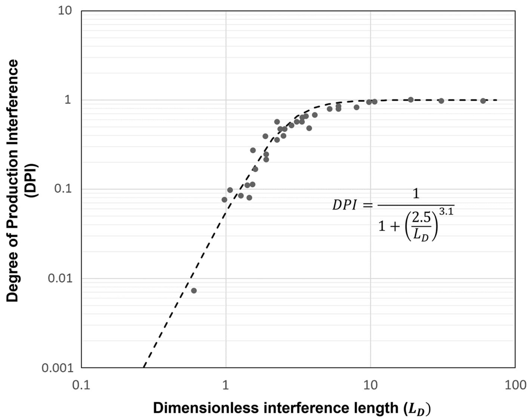
Fig. 5: The relationship between \(LD\) and \(DPI\) from numerical simulations collapse onto a curve represented by the dashed line. The dots represent the individual numerical simulations. The simulations have varying fracture, fluid and matrix property inputs.
3. Understanding DPI for Unbounded vs Bounded Wells
A DPI of 100% relates to a doubling of production rate of a well when an adjacent (offset) well is shut in. For two wells that are unbounded on the outside, the DPI cannot exceed 100%, because an offset well can only influence production on one side of its neighbor.
The DPI formulation presented by Almasoodi et al. (2023) assumes a specific configuration: two wells unbounded on either side with symmetric fracture geometries. This assumption limits how much interference a neighboring well can exert.
To quantify production interference, it is useful to define the Fractional Production Loss (FPL):
or, equivalently:
For example, a DPI of 100% coressponds to an FPL of 0.5, indicating a 50% loss in production due to interference from the neighboring well.
However, when a well is bounded on either side (e.g., part of a uniformly spaced well pattern), the interference from neighboring wells can be more severe. In such cases, FPL can exceed 0.5, resulting in DPI values much greater than 100%.
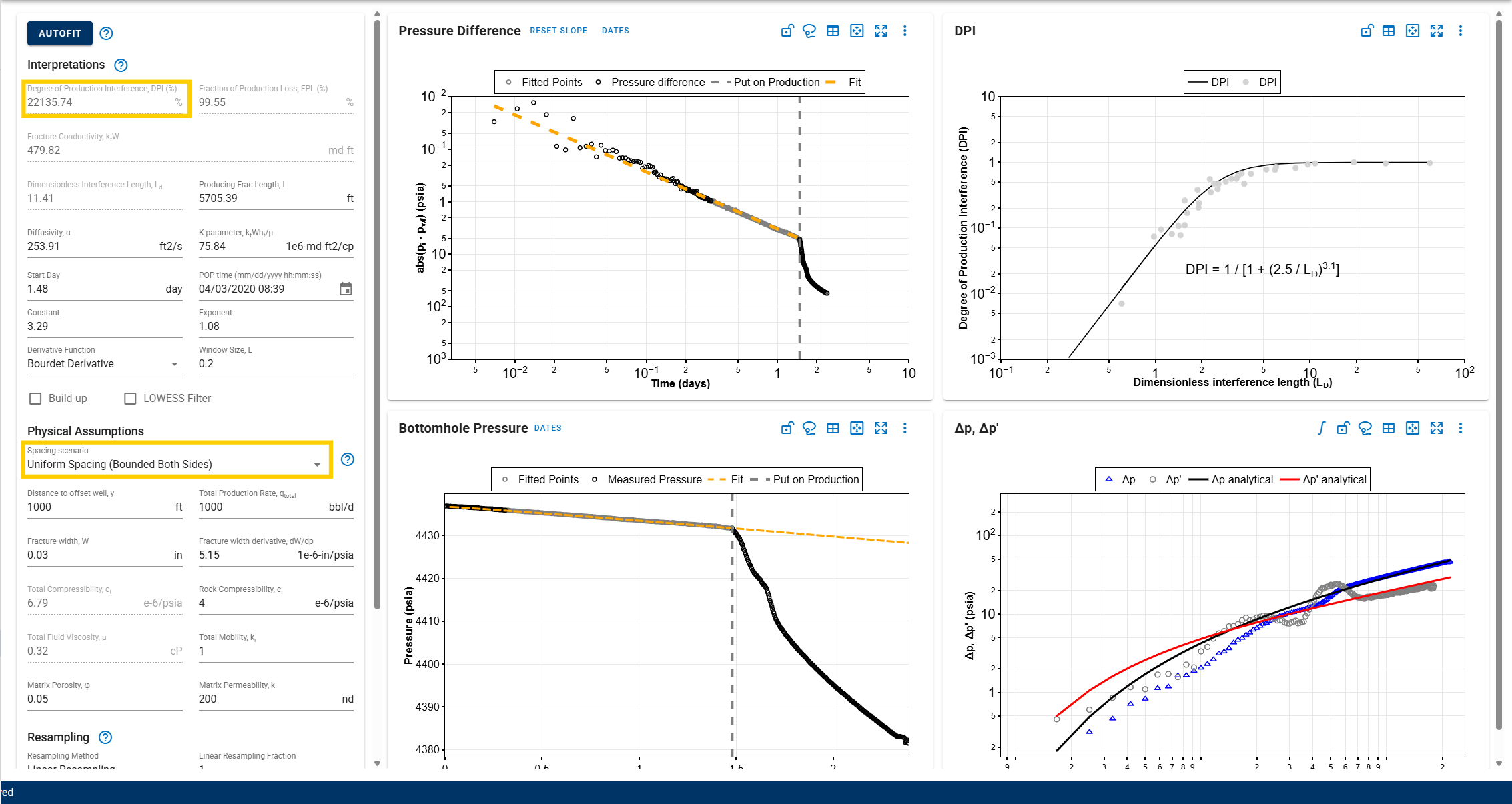
In the software, selecting Uniform Spacing (Bounded Both Sides) allows for scenarios where DPI >> 100%. As shown in the case above, DPI can reach values as high as ~22,000% when the calculated FPL is significantly greater than 0.5.
DQI Workflow
Before Getting Started
Recommended Data Size for DQI Tests
DQI datasets could be far higher frequency than needed. Datasets can vary from second by second frequency to tens of seconds for the entirety of the test. This can be harder to handle, and make the numerical derivative calculation unweildy.
Rather than uploading high-resolution data, we recommend resampling the dataset externally using pressure increments of 5 to 10 psi. This reduces file size and improves performance. For best results, keep the number of uploaded data rows between 30,000 and 40,000. To learn how to resample your data within whitson+, see the resampling section here.
Data Truncation
The Truncate Data feature in the Well Test modules (CPG and DQI) allows users to remove unwanted portions of the dataset and focus the analysis on a specific time range. This is useful for excluding early-time noise, late-time operational changes, or any data outside the period of interest.
Truncation Methods
-
Date-Based Truncation
Users can manually define the truncation window by selecting a truncate start date and truncate end date using the calendar controls. All data outside the selected range is removed.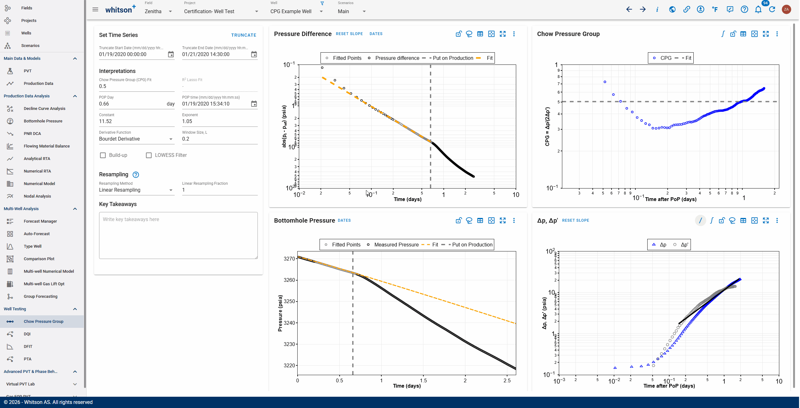
-
Visual Truncation
Users can visually select the data range to retain directly on the plot. A black dotted line marks the start of the retained data, and a blue dotted line marks the end. Data before the black line and after the blue line will be deleted.
DQI Dataset Example
Here's an example DQI dataset.
Example DQI Dataset
Courtesy: Devon, Resfrac.
Create a Project
- Go to the Projects module in the navigation panel.
- Click ADD PROJECT up to the right.
- Name the project "your name - DQI Example Certificate".
- Click SAVE.
- Click MASS UPLOAD up to the right.
- Upload the DQI Example Well Excel file. You can also switch to the examples tab and click Upload on the Well Test Certificate.
- Click SAVE.
- All steps are shown in the .gif above.
You can also upload your own pressure interference dataset if you'd like. Ensure that the pressure measurements are in the pwf or gauge pressure column and the same Well Name exists on the Well Data sheet.
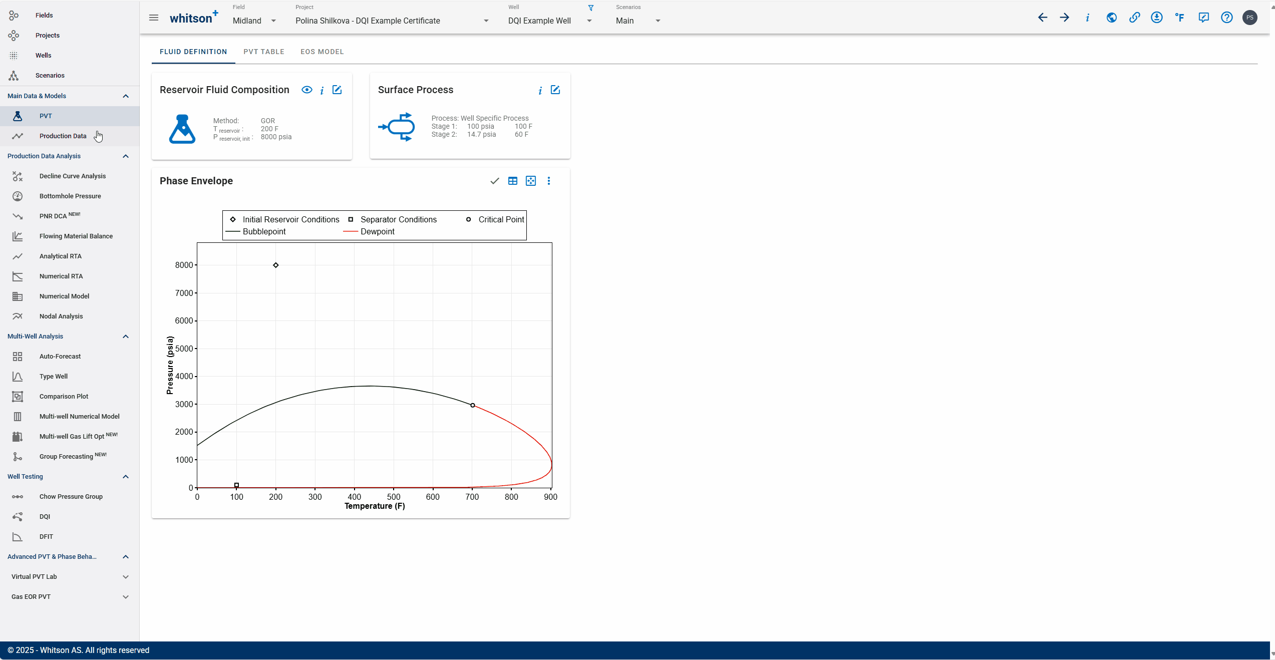
PVT
You need PVT initialization to gather fluid properties like fluid compressibility, viscosity, etc. from the black oil tables. You want to ensure that the PVT initialization matches the fluid that can be expected between these wells.
- Go to the Scenarios module in the navigation panel.
- Initialize PVT with 100% water saturation
- Go to the PVT module in the navigation panel.
- Open the Reservoir Fluid Composition Input Card
- Click SAVE.
- All steps are shown in the .gif above.
For a DQI test shortly after the initial stimulation in the offset well prior to the well being produced, initialize PVT with 100% water saturation - this is what we'll do here in this example dataset, as shown in the GIF above.
For tests where the well pair has been producing hydrocarbons, initialize the PVT with the GOR associated with the reservoir fluid in place.
Align the POP Line of the Offset Well
- Go to the Production Data module in the navigation panel.
- Taking a quick look at the pressures in the production data.
- Go to the DQI section in the Well Testing module in the navigation panel.
- Set the offset well POP to 1.48 days.
- All steps are shown in the .gif above.
You can enter it in or move the vertical dashed line graphically to the point in time when the offset well is POP'ed.
Align the Line to Pressure Trend Before POP
- Fit the prior pressure trend by moving and adjusting the slope line to align with the stabilized pressure trend prior to POP.
- You can do this manually or you can just lasso fit the stabilized pressure data.
- All steps are shown in the .gif above.
Notice how the pressure and pressure derivative vs time after POP plot is dynamically recalculated as you make adjustments to the prior pressure trend.
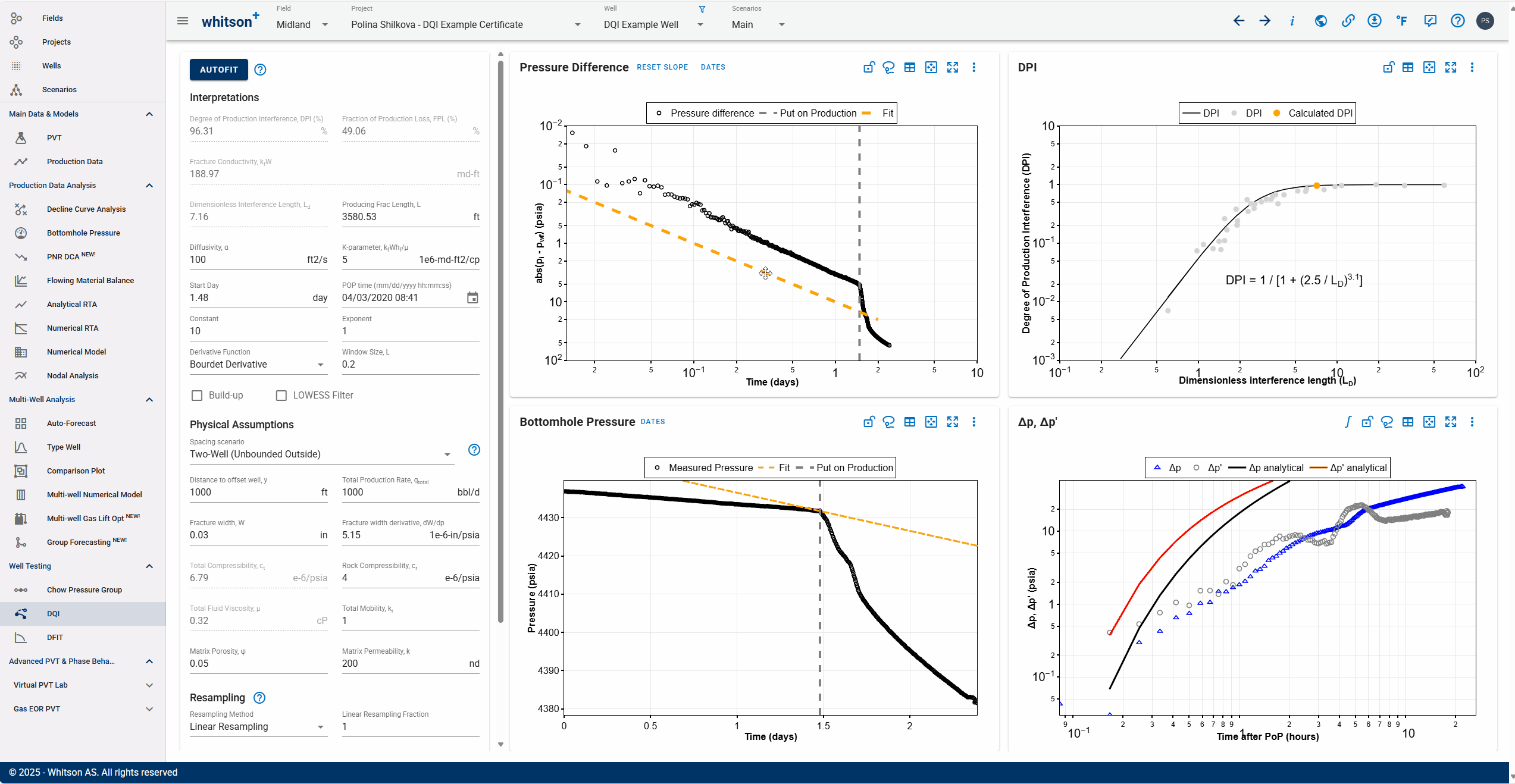
Autofit
Once the prior pressure trend and POP is picked, we have a plot of.
- Click the AUTOFIT button (off to the top-left of the page)
-
This fits the analytical model to the pressure and pressure derivative data to determine model parameters:
- α (controls hydraulic diffusivity) - impacts the timing of the onset of pressure interference.
- κ (controls fracture conductivity) - impacts the shape of the curve after the interference. Resolving these two parameters allows you to calculate the fracture conductivity 'κ' and maximum possible drainage length along the fracture, 'L', given W (fracture width or aperture) and (change in fracture aperture with change in pressure) and other parameters.
Assessing fit quality
The priority is to ensure that the fit matches the initial response - the first 10s or 100s of psi. The analytical solution is not expected to match the transient after the initial response.
-
Then the Ld is calculated, given the well spacing, 'y'.
- This is plotted in the empirical correlation developed to calculate DPI, given the .
- The resulting DPI should be close to 95%.
- All steps are shown in the .gif above.
Note down the α and κ, both of which are indicators of good or bad well-pair connectivity, apart from the DPI. This will help you rank the well-pair connectivity on large scale tests with multiple well pairs
References
Mouin Almasoodi\(^1\), Thad Andrews\(^1\), Curtis Johnston\(^1\), Mark McClure\(^2\), and Ankush Singh\(^2\)(2023). A new method for interpreting well‑to‑well interference tests and quantifying the magnitude of production impact: theory and applications in a multi‑basin case study.\(^1\)Devon Energy, \(^2\)ResFrac Corporation.
Zimmerman RW (2018) Pressure diffusion equation for fluid flow in porous rocks. Imp Coll Lect Pet Eng 25:1–21.
Horne RN (1995) Modern Well Test Analysis: A Computer-aided Approach.
Hetnarski RB et al (2014) Encyclopedia of thermal stresses. Springer, Dordrecht.